CMS-Flow Numerical Methods: Difference between revisions
No edit summary |
|||
| (33 intermediate revisions by 2 users not shown) | |||
| Line 1: | Line 1: | ||
= Overview = | = Overview = | ||
CMS-Flow has both implicit and explicit solution schemes. The explicit solver is designed for dynamic problems with extensive wetting and drying that require small computational time-steps, while the implicit solver is intended for simulating tidal- and wave-induced circulation at tidal inlets, navigation channels, and adjacent beaches. A detailed description of the numerical formulation of the explicit solver of CMS-Flow can be found in Buttolph et al. (2006) and is not repeated here. The sections below specifically refer to the implicit solver of CMS-Flow. | CMS-Flow has both implicit and explicit solution schemes. The explicit solver is designed for dynamic problems with extensive wetting and drying that require small computational time-steps, while the implicit solver is intended for simulating tidal- and wave-induced circulation at tidal inlets, navigation channels, and adjacent beaches. A detailed description of the numerical formulation of the explicit solver of CMS-Flow can be found in Buttolph et al. (2006) and is not repeated here. The sections below specifically refer to the implicit solver of CMS-Flow. | ||
The implicit solver uses the SIMPLEC ( | |||
The implicit solver uses the SIMPLEC (<u>S</u>emi-<u>I</u>mplicit <u>M</u>ethod for <u>P</u>ressure <u>L</u>inked <u>E</u>quations <u>C</u>onsistent) algorithm (van Doormal and Raithby 1984) on a non-staggered grid to handle the coupling of water level and velocity. Primary variables u-, v-velocity, and water level are stored on the same set of grid points, and fluxes at cell faces are determined using a Rhie and Chow (1983) type momentum interpolation method (Wu et al. 2011). The explicit solver uses a staggered grid with velocities at the cell faces and the water levels and water depths at the cell centers (Buttolph et al. 2006). CMS-Flow also calculates salinity, sediment transport, and morphology change. The governing equations for hydrodynamics and sediment and salinity transport have similar forms which can be written as a general transport (advection-diffusion) equation. In order to avoid redundant derivations of discretized equations, the discretization of the general transport equation is described in this chapter, and the same discretization may be applied to all of the transport equations. Then, the specific solution procedures for hydrodynamics, sediment transport, and bed change are introduced. | |||
==CMS-Flow Computational Grid== | ==CMS-Flow Computational Grid== | ||
The implicit version of CMS-Flow | The explicit time scheme in CMS-Flow supports uniform and non-uniformly spaced Cartesian grids while the implicit version of CMS-Flow supports generic Cartesian grids which can be uniform, non-uniform, or telescoping. The telescoping locally refines the mesh by splitting a cell into subcells. The only requirement imposed by the numerical methods is that the cells must have a rectangular shape. Additional requirements are imposed by the user interface which limits the variety of types of Cartesian grids to help simplify the grid generation and avoid grid quality issues. The following requirements are applied: | ||
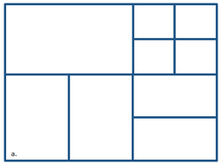
:1. Cells can only be subdivided into four subcells. | |||
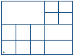
:2. Only two neighboring cells are allowed in the same direction (i.e., north, south, east, and west). | |||
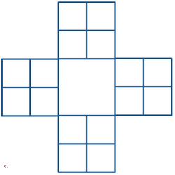
:3. Cells may have a maximum of six neighbors. | |||
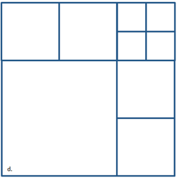
:4. Refinement levels must be spaced by at least one cell apart (i.e., cells that share the same corner must be one refinement level apart). | |||
Examples of violations of the above four requirements are shown in sequential order in Figure 1 from a to d. Limiting the number of neighboring cells to six avoids excessive cell refinement and limits the band width of the coefficient matrix for the linearlized system of equations solved by the implicit solution scheme. The last two requirements avoid having excessive cell refinement which can cause numerical instabilities. The first requirement simplifies the grid generation process but may be relaxed in future versions. The last requirement is enforced for grid quality purposes and a more smoothly varying grid resolution. | |||
<br style="clear:both" /> | |||
<center> | |||
[[File:fig_3_1_a.bmp|250px]] [[File:fig_3_1_b.bmp|250px]] | |||
[[File:fig_3_1_c.bmp|250px]] [[File:fig_3_1_d.bmp|250px]] | |||
'''Figure 1. Examples of Invalid Cartesian computational grids''' | |||
</center> | |||
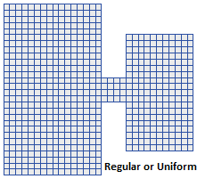
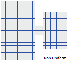
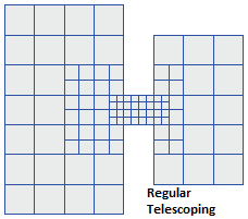
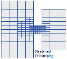
The CMS-Flow grids generated in the SMS interface can be classified as uniform, non-uniform Cartesian grids, regular telescoping, and stretched telescoping grids (Figure 2). | |||
<center> | |||
[[File:fig_3_2_a.bmp]] [[File:fig_3_2_b.bmp]] | |||
[[File:fig_3_2_c.bmp]] [[File:fig_3_2_d.bmp]] | |||
'''Figure 2. Types of Cartesian grids supported by the SMS interface and CMS-Flow.''' | |||
</center> | |||
: | One important aspect of incompressible flow models is the location of primary variables: velocity and pressure (water level). On a staggered grid, the pressure (water level) is located at the center of cells and the u- and v-velocities are located along the faces of cells (Harlow and Welsh 1965; Patankar 1980). On a non-staggered grid, all of the primary variables are located at the center of cells. This can lead to the spatial oscillations referred to as checkerboard oscillations and model instability if the linear interpola-tion between nodes is used to determine the fluxes at cell faces. A staggered grid can more easily eliminate these oscillations when compared to a non-staggered grid; however, a non-staggered grid involves a simpler source code and can minimize the number of coefficients that must be computed and stored during a simulation because many of the terms in the equations are equal. In particular, a staggered grid is more complicated when handling the interface between coarse and fine cells where 5- or 6-face control volumes are used. Therefore, a non-staggered (collocated) grid approach is adopted for CMS-Flow with a Rhie and Chow (1983) momentum interpolation technique used to eliminate the checkerboard oscillations. Figure 3 shows the location of primary variables on the 5- and 7-point stencils (computational molecule). | ||
<center> | |||
[[File:fig_3_1_a.png|300px]] [[File:fig_3_1_b.png|300px]] | |||
'''Figure 3. Computational stencils and control volumes for two types of Cartesian grids: non-uniform Cartesian (left) and telescoping grid (right).''' | |||
</center> | |||
Computational cells are numbered in an unstructured manner via a | The data structure for a grid can be approached in three ways: 1) block-structured, 2) hierarchical tree, and 3) unstructured. The block-structured approach divides the domain into multiple blocks, and each block is treated as structured. The block structured approach requires a special treatment between blocks to ensure mass and momentum balance using this approach. The hierarchical tree approach is memory intensive and requires parent-child relationships and a tree traverse to determine mesh connectivity. For the unstructured approach, all cells are numbered in a 1D sequence, and tables are used to determine the connectivity of neighboring cells. Among these three approaches, the unstructured approach is the most simple and is therefore applied in CMS-Flow. Computational cells are numbered in an unstructured manner via a 1D index array. Inactive cells (permanently dry) are not included in the 1D index array to save memory and computational time. All active computational cells are numbered sequentially. It is noted that using an unstructured data approach does not limit the model from using matrix solvers designed for structured grids. For convenience with handling boundary conditions, each boundary cell has a neighboring ghost cell outside of the computational domain. | ||
=General Transport Equation= | =General Transport Equation= | ||
{{Equation| | {{Equation| | ||
<math> | <math> | ||
\underbrace { | \underbrace { \frac {\partial}{\partial t}\left(\frac{h\phi}{\beta}\right) | ||
}_{\text {Temporal Term}} | }_{\text {Temporal Term}} | ||
+ \underbrace {\frac{\partial(hV_j \phi)} {\partial x_j} }_{\text{Advection Term}} | + \underbrace {\frac{\partial(hV_j \phi)} {\partial x_j} }_{\text{Advection Term}} | ||
| Line 32: | Line 61: | ||
\frac{\partial}{\partial x_j} \left(\Gamma h \frac{\partial \phi}{\partial x_j} \right) | \frac{\partial}{\partial x_j} \left(\Gamma h \frac{\partial \phi}{\partial x_j} \right) | ||
}_{\text{Diffusion Term}} | }_{\text{Diffusion Term}} | ||
+ \underbrace{ | + \underbrace{S}_{\text{Source Term}} | ||
</math> | </math> | ||
|1}} | |1}} | ||
where <math>\phi</math> | |||
where: | |||
::<math>\phi</math> = general scalar | |||
::''h'' = total water depth [m] | |||
::<math>\beta</math> = correction factor [-] | |||
::<math>V_j</math> = total flux velocity [m/s] | |||
::<math>\Gamma</math> = diffusion coefficient for <math>\phi</math> [<math>m^2 /s</math>] | |||
::S = source/sink term which includes all remaining terms. | |||
Note that in the case of the continuity and momentum equations, <math>\phi</math> is equal to 1 and <math>V_i</math>respectively. In the case of sediment and salinity transport, <math>\phi</math> is equal to <math>C_{tk}</math> and <math>C_{sal}</math>, respectively. The correction factor (''β'') is equal to the total-load correction factor and equal to 1 for all other equations. | |||
==Spatial Discretization== | ==Spatial Discretization== | ||
A control-volume technique is used in which the governing equations are integrated over a control volume to obtain an algebraic equation that can be solved numerically. Integration of Equation ( | |||
A control-volume technique is used in which the governing equations are integrated over a control volume to obtain an algebraic equation that can be solved numerically. Integration of Equation (1) over a control volume yields: | |||
{{Equation| | {{Equation| | ||
<math> | <math> | ||
\int_A \frac {\partial( | \int_A \frac {\partial}{\partial t}\left(\frac{h_\phi}{\beta} \right) dA + \int_A \frac {\partial}{\partial x_j}\left(hV_j \phi - \Gamma h\frac{\partial \phi}{\partial x_j} \right)dA = \int_A SdA | ||
</math> | </math> | ||
|2}} | |2}} | ||
| Line 48: | Line 88: | ||
{{Equation| | {{Equation| | ||
<math> | <math> | ||
\frac {\partial (h_P \phi_P | \frac {\partial}{\partial t}\left(\frac{h_P \phi_P}{\beta_P} \right) \Delta A_P + \oint_L h[(\hat{n_i}V_i)\phi - \Gamma(\hat{n_i}\bigtriangledown_i \phi)]dL = S_P \Delta A_p | ||
</math> | </math> | ||
|3}} | |3}} | ||
| Line 54: | Line 94: | ||
{{Equation| | {{Equation| | ||
<math> | <math> | ||
\frac {\partial (h_P \ | \frac {\partial}{\partial t}\left(\frac{h_P \phi_p}{\beta_p} \right) \Delta A_P + | ||
\sum_f h_f \left [ | \sum_f h_f \left [V_f \phi_f - \Gamma_f(\bigtriangledown_\perp \phi)_f \right]\Delta l_f = S_P \Delta A_p | ||
</math> | </math> | ||
|4}} | |4}} | ||
| Line 61: | Line 101: | ||
where | where | ||
::<math>\hat{n_i} = (\hat{n_1} , \hat{n_2})</math> = outward unit vector normal to cell face ''f'' | ::<math>\hat{n_i} = (\hat{n_1} , \hat{n_2})</math> = outward unit vector normal to cell face ''f'' [-] | ||
::<math>V_f = (\hat{n_i}V_i)_f</math> = outward cell face velocity | ::<math>V_f = (\hat{n_i}V_i)_f</math> = outward cell face velocity [m/s] | ||
:: | ::::::<math>\phi_P</math> = value of <math>\phi</math> at the cell centroid | ||
::<math>(\bigtriangledown_\perp \phi)_f = (\hat{n_i}\bigtriangledown_i \phi)_f</math> | ::::::''<math>h_P</math>'' = total water depth at the cell face centroid [m] | ||
::::::<math>h_f</math> = interpolated total water depth at cell face f [m] | |||
:::<math>(\bigtriangledown_\perp \phi)_f</math> = outward normal gradient of <math>\phi</math> at cell face ''f:''<math>\ (\bigtriangledown_{\perp} \phi)_f = (\hat{n_i}\bigtriangledown_i \phi)_f</math> | |||
::::::<math>\Gamma_f</math> = interpolated diffusion coefficient for <math>\phi</math> | |||
:::::<math>\Delta A_P</math> = area of cell P [m/s] | |||
::::::<math>\Delta l_f</math> = length of cell face f [m] | |||
::::::<math>S_P</math> = source/sink term. | |||
In the above equations, the Gauss Divergence Theorem has been used to convert the area integral to a boundary integral. In addition, the area ingegrals have been evaluated assuming variable vary linearly within cells. The cell face velocity,<math>(V_f)</math> , is calculated using a momentum interpolation method similar to that of Rhie and Chow (1983) and is described in ''Hydrodynamics'' of the present Chapter. | |||
==Temporal Discretization== | ==Temporal Discretization== | ||
The general transport equation is rewritten as | The general transport equation is rewritten as | ||
{{Equation| | |||
{{Equation|<math> | |||
\ | \frac {\partial}{\partial t} \left(\frac{h\phi}{\beta} \right)= \hat{G}</math>|5}} | ||
</math> | |||
|5}} | where <math>\hat{G}</math> includes all the remaining terms. For stability and efficiency, a fully implicit time-stepping scheme is used in the form | ||
where includes all the remaining terms, such as …. For stability and efficiency, a fully implicit time-stepping scheme is used in the form | where includes all the remaining terms, such as …. For stability and efficiency, a fully implicit time-stepping scheme is used in the form | ||
where <math>\theta</math> is a weighting factor between 0 and 1. For <math>\theta = 0</math>, the scheme reduces to the first-order backward Euler scheme, and with <math>\theta = 1</math>, the scheme reduces to the second-order backward scheme (Ferziger and Peric 1997). The superscripts indicate the time step levels, with n+1 being the | {{Equation|<math> | ||
\frac{1}{\Delta t}\left[(1 + 0.5\hat{\theta)}\frac{h^{n+1}\phi^{n+1}}{\beta^{n+1}} - (1+\hat{\theta}) \frac{h^n \phi^n}{\beta^n} + 0.5\hat{\theta}\frac{h^{n-1}\phi^{n-1}}{\beta^{n-1}} \right] = \hat{G}^{n+1} | |||
</math>|6}} | |||
where <math>\hat{\theta}</math> is a weighting factor between 0 and 1. For <math>\hat{\theta} = 0</math>, the scheme reduces to the first-order backward Euler scheme, and with <math>\hat{\theta} = 1</math>, the scheme reduces to the second-order backward scheme (Ferziger and Peric 1997). The superscripts indicate the time step levels, with n+1 being the next time-step and ''n'' being the previous time-step. | |||
==Cell-face Interpolation Operator== | |||
The general formula for estimating the cell-face value <math>\phi_f</math>is given by | |||
{{Equation|<math> | |||
{ | |||
<math> | |||
\phi_f = f_\perp \phi_N + (1-f_\perp)\phi_P + f_\perp(r_\parallel \bigtriangledown_\parallel \phi)_N + (1-f_\perp) | \phi_f = f_\perp \phi_N + (1-f_\perp)\phi_P + f_\perp(r_\parallel \bigtriangledown_\parallel \phi)_N + (1-f_\perp) | ||
(r_\parallel \bigtriangledown_\parallel \phi)_P | (r_\parallel \bigtriangledown_\parallel \phi)_P | ||
</math> | </math>|7}} | ||
|7}} | |||
where <math>f_\perp</math> is a linear interpolation factor, <math>\bigtriangledown_\parallel </math> is the gradient operator in the direction parallel to face ''f'', and <math>r_\parallel</math> is the distance from the cell center to the ghost point ''(O)'' parallel to the cell face ''(f)'' (see Figure 4). | |||
<center> | |||
[[File:fig_4.bmp|600px]] | |||
'''Figure 4. Schematic showing interface interpolation: (a) coarse to fine and (b) fine to coarse.''' | |||
</center> | |||
The subscripts <math>\|</math> and <math>\perp</math> indicate the components parallel and normal to the cell face. By definition,<math>\| = 2|\hat{n_1}| + 1|\hat{n_2}| \text{ and }\perp = 1|\hat{n_1}| + 2|\hat{n_2}|</math> . Note that for neighboring cells without any refinement, <math>r_\|</math> is equal to zero and the above equation is consistent with non-refined cell faces. The linear interpolation factor is defined as | |||
{{Equation| | {{Equation| | ||
<math> | <math> | ||
| Line 110: | Line 171: | ||
where <math>x_{\perp ,f}</math> is the coordinate of ''f'' perpendicular to the face and <math>\Delta x_\perp</math> is the cell dimension perpendicular to the face ''f''. | where <math>x_{\perp ,f}</math> is the coordinate of ''f'' perpendicular to the face and <math>\Delta x_\perp</math> is the cell dimension perpendicular to the face ''f''. | ||
== | ==Cell-face Gradient== | ||
A linearly exact second-order approximation for the normal gradient at cell face ''f'' is calculated using the auxiliary node concept of Ferziger and Peric (1997): | |||
{{Equation| | |||
<math> | {{Equation|<math> | ||
\ | (\bigtriangledown_{\perp}\phi)_f = \frac{\phi_N - \phi_P}{|\delta_{\perp}|} + \frac{(r_\|\bigtriangledown_\|\phi)_N - (r_\|\bigtriangledown_\|\phi)_P} {|\delta_{\perp}|} | ||
\ | </math>|9}} | ||
\ | |||
where the subscripts ''P'' and ''N'' refer to two neighboring cells, <math>|\delta_{\perp}| = |x_{\perp,N} - x_{\perp,P}| </math> is the distance between cells P and N, normal to the cell face (Figure 4), and <math>\bigtriangledown_\|</math> is the gradient operator in the direction parallel to face ''f''. Ham et al. (2002) compared the auxiliary node formulation to the fully-unstructured discretization proposed by Zwart et al. (1998) for the viscous terms and found that the auxiliary node formulation is significantly more stable. | |||
==Cell-centered Gradient== | |||
The cell-centered gradient operator is calculated using the Gauss’ Divergence Theorem as | |||
{{Equation|<math> | |||
\int_A \bigtriangledown_i \phi dA = \sum_f \hat{n_i}\phi_f \Delta l_f</math>|10}} | |||
The equation above is second order and conservative for regular and non-uniform grids. | |||
The | |||
==Reconstruction, Monotonicity, and Slope Limiters== | |||
Variables are linearly reconstructed within the cells as | |||
{{Equation|<math> | |||
{{Equation| | \phi = \phi_P + \overrightarrow{r}\cdot \bigtriangledown \phi_P | ||
<math> | </math>|11}} | ||
\ | |||
</math> | |||
| | |||
where <math>\ | where <math>\phi_P</math> is the cell-average value specified at the cell centroid, <math>\overrightarrow{r}</math> is the distance vector from the cell centroid to any location within the cell, and <math>\bigtriangledown \phi_P</math> is the cell-centered gradient. The reconstruction is second order and conservative in the sense that <math>\phi_P \Delta A_P = \int_A \phi dA</math>. The linear reconstruction is used when interpolating cell-face values (Equation 7) and calculating cell-face gradients (Equation 13). If the reconstruction satisfies the local maximum principle | ||
{{Equation|<math> | |||
min(\phi - \phi_P,0) \leq \overrightarrow{r}\cdot \bigtriangledown \phi_P \leq max(\phi - \phi_P,0) | |||
</math>|12}} | |||
then no new extrema are created within the cell, and the solution is monotonic. Figure 5 shows two examples of linear reconstruction with and without slope limiters to ensure monotonicity. | |||
<center> | |||
[[File:fig_5.bmp|500px]] | |||
'''Figure 5. Schematics showing examples of (a) non-limited and (b) limited linear reconstructions.''' | |||
</center> | |||
</ | |||
For non-telescoping grids, the slope limiter is calculated as | |||
{{Equation|<math> | |||
\Phi(R) = \left\{\begin{align} | |||
&\frac {4R} {(R+1)^2}\quad van Leer (1979) \\ | |||
&\frac {2R} {(R^2 +1)}\quad van Albada \ et\ al.\ (1982) \\ | |||
&min \left(1, \frac{4}{R+1}, \frac {4R} {R+1} \right) \quad MUSCL (van Leer 1979) | |||
\end{align}\right. | |||
</math>|13}} | |||
where R is the ratio between two consecutive slopes | |||
{{Equation|<math> | |||
R = \frac {(\phi_{i+1}-\phi_i)(x_i - x_{i-1} ) } {(x_{i+1}-x_i)(\phi_i -\phi_{i-1})}</math>|14}} | |||
Here, the second-order van Leer (1979) limiter is used because of its smoothness. Figure 6 shows a comparison of three different common limiters. The slope limiter is applied in each direction separately. | |||
<center> | |||
< | |||
[[File:fig_3_6a.bmp|400px]] | |||
Figure | '''Figure 6. Comparison of three different slope limiters.''' | ||
</center> | |||
For | For unstructured grids the slope limiters described above are difficult to implement because of the difficulty in defining forward and backward differences. For telescoping grids the following Limited Central Difference (LCD) slope limiting procedure of Hubbard (1999) is applied: | ||
{{Equation|<math>\Phi_f = | |||
\Phi_f = | \left\{\begin{align} | ||
\left\{ | |||
\begin{align} | |||
&\frac {max(\phi_N - \phi_P , 0)} | &\frac {max(\phi_N - \phi_P , 0)} | ||
{\overrightarrow{r | {(\overrightarrow{r}\cdot \bigtriangledown \phi)_P} | ||
&for \overrightarrow{r | &for\ (\overrightarrow{r}\cdot \bigtriangledown \phi)_P > max(\phi_N - \phi_P,0) \\ | ||
&\frac{min(\phi_N - \phi_P , 0)} | &\frac{min(\phi_N - \phi_P , 0)} | ||
{\overrightarrow{r | {(\overrightarrow{r}\cdot \bigtriangledown \phi)_P} | ||
&for \overrightarrow{r | &for\ (\overrightarrow{r}\cdot \bigtriangledown \phi)_P < min(\phi_N - \phi_P,0) \\ | ||
&1&otherwise \\ | &1&otherwise\\ | ||
\end{align} | \end{align}\right.</math>|15}} | ||
\right. | |||
</math> | where <math>\overrightarrow{r}_{p} = \overrightarrow{x}_f - \overrightarrow{x}_p</math>. In the procedure outlined by Hubbard (1999), a scalar limiter is then calculated as <math>\Phi = min(\Phi_f)</math>. Here, a directional limiter is applied as <math>\phi_{i} = \min\limits_{\textit{f} \in \textit{f} \perp i} (\phi_f) </math>, which is less dissipative. Finally, the cell-centered gradient is limited as | ||
{{Equation|<math>\bigtriangledown_i \phi_P = \Phi_i \bigtriangledown_i^* \phi_P</math>|16}} | |||
where <math>\bigtriangledown_i^* \phi_P</math> is the unlimited gradient. | |||
==Advection Schemes== | |||
===Hybrid Scheme=== | |||
The hybrid scheme is composed of a first-order upwind scheme and a second-order central difference scheme. The cell-face advective value is given by | |||
{{Equation|<math>\phi_f = | |||
\left\{\begin{align} | |||
&(\phi_D + \phi_C) / 2 | |||
&for\ |P_f| > 2 \\ | |||
&\phi_c | |||
&for\ |P_f| >2 | |||
\end{align}\right. </math>|17}} | |||
where the subscripts ''D'' and ''C'' indicate the downstream and upstream values, and <math>P_f = V_f|\delta_{\perp}| / \Gamma_f</math> is the Peclet number at the cell face in which ,<math>|\delta_{\perp}| = |x_{\perp,N} - x_{\perp,P}|</math>. In the hybrid scheme, when the Peclet number is larger than 2, the first-order upwind value is used; otherwise, the second-order central difference value is used. | |||
===Exponential Scheme=== | |||
The exponential scheme interpolates the face value using an exact solution to the 1D steady advection-diffusion equation: | |||
{{Equation|<math>\frac{\phi_f - \phi_p}{\phi_N - \phi_P} = \frac{exp(P_f f_{\perp})-1}{\exp(P_f)-1} | |||
</math>|18}} | |||
The exponential scheme has automatic upwinding and is stable but is usually less than second order. | |||
===Hybrid Linear/Parabolic Scheme=== | |||
The Hybrid Linear/Parabolic Approximation (HLPA) scheme of Zhu (1991) may be written as | |||
{{Equation|<math>\phi_f = \left\{ | |||
\begin{align} | |||
&\phi_c + (\phi_D - \phi_C)\hat{\phi_C}, | |||
&for\ 0 \leq \hat{\phi_C} \leq 1 \\ | |||
&\phi_C | |||
&otherwise | |||
\end{align}\right.</math>|19}} | |||
where the subscripts ''D'', ''C'', and ''U'' indicate the first downstream and first and second upstream cells, respectively. The normalized variable <math>(\hat{\phi_C}</math>) is determined based on the formulation of Jasak et al. (1999) | |||
{{Equation|<math>\hat{\phi_C} = \frac{\phi_C - \phi_U}{\phi_D - \phi_U} = 1 - \frac{\phi_D - \phi_C}{2(\bigtriangledown_{\perp}\phi)_C \delta_{\perp,C}}</math>|20}} | |||
where <math>\ | where <math>\delta_{\perp,C} = x_{\perp,D} - x_{\perp,C}</math>. The HLPA scheme is second order. Choi et al. (1995) found that the HLPA scheme has similar accuracy to the third-order SMARTER (<u>S</u>harp and <u>M</u>onotonic <u>A</u>lgorithm for <u>R</u>ealistic <u>T</u>ransport <u>E</u>fficiently <u>R</u>evised) and LPPA (<u>L</u>inear and <u>P</u>iecewise-<u>P</u>arabolic <u>A</u>pproximation) schemes but is simpler and more efficient (Shin and Choi 1992; Choi et al. 1995). | ||
== Source/sink | == Source/sink Term == | ||
The source/sink term is linearized as (Patankar 1980) | The source/sink term is linearized as (Patankar 1980) | ||
{{Equation|<math>S_P = S_P^C + S_P^P \phi_P</math>|21}} | |||
</math> | |||
The coefficient <math>S_P^P</math> is required to be non-positive for stability. | |||
== Assembly of Algebraic Equations == | == Assembly of Algebraic Equations == | ||
| Line 267: | Line 311: | ||
{{Equation|<math> | |||
a_P \phi_P^{n+1} = \sum_N a_N \phi_N^{n+1} + | a_P \phi_P^{n+1} = \sum_N a_N \phi_N^{n+1} + b </math>|22}} | ||
</math> | |||
where the subscript ''N'' refers to the neighboring cell sharing cell face, <math>a_P</math> | where the subscript ''N'' refers to the neighboring cell sharing cell face, <math>a_P</math> and <math>a_N</math> are linear coefficients for <math>\phi_P^{n+1}</math> and <math>\phi_N^{n+1}</math> . The last term, ''(b)'' contains all the remaining terms. Applying a similar equation for all of the internal cells of a grid results in a system of algebraic equations. This set of equations are referred to as the discretized governing equations. | ||
== Implicit Relaxation == | == Implicit Relaxation == | ||
The right-hand side of the algebraic system of equations ''(b)'' generally contains deferred corrections and source terms which must be computed iteratively. This iteration loop is referred to as the outer loop, and the loop within the linear iterative solver (see Section ''Iterative Solvers'') is referred to as the inner loop. Under-relaxation is often applied to stabilize the convergence of the outer iteration loop. Under-relaxation may be applied as <math>\phi^{m+1} = a_\phi \phi^{n+1} + (1 - a_\phi)\phi^m</math> in which <math>a_\phi</math> is an under-relaxation parameter <math>(0 < a_\phi \leq 1)</math>. The superscript m indicates the previous iteration, and superscript ''m+1'' indicates the new relaxed value. A better approach is used here to introduce the under-relaxation directly in the algebraic system of equations (Majumdar 1988; Ferziger and Peric 1997) as | |||
</math>( | |||
{{Equation|<math> | |||
\frac {a_P}{\alpha_\phi}\phi_P^{n+1} = \sum_N a_N \phi_N^{n+1} + b + \frac {1-\alpha_\phi} {\alpha_\phi} a_P \phi_P^m | |||
</math>|23}} | |||
This is referred to implicit under-relaxation and has the effect of making the coefficient matrix more diagonally dominant, thus improving convergence. | |||
== Iterative Solvers == | == Iterative Solvers == | ||
The selection of an iterative solver is one key issue concerning the overall per-formance of the model. CMS has three iteration solvers available and they are described in more detail below: 1) GMRES variation, 2) BiCGStab, and 3) Gauss-Seidel. The default iterative solver for CMS is a variation of the GMRES ( | The selection of an iterative solver is one key issue concerning the overall per-formance of the model. CMS has three iteration solvers available and they are described in more detail below: 1) GMRES variation, 2) BiCGStab, and 3) Gauss-Seidel. The default iterative solver for CMS is a variation of the GMRES (<u>G</u>eneralized <u>M</u>inimum <u>RES</u>idual) method (Saad 1993) and is used to solve the algebraic equations. The original GMRES method (Saad and Schultz 1986) utilizes the Arnoldi process to reduce the coefficient matrix to the Hessenburg form and minimizes the norm of the residual vector over a Krylov subspace at each iterative step. The variation of the GMRES method recommended by Saad (1993) allows changes in preconditioning at every iteration step. An Incomplete LU Factorization (ILUT; Saad, 1994) is used as the preconditioner to speed-up convergence. The GMRES solver is applicable to symmetric and non-symmetric matrices and leads to the smallest residual for a fixed number of iterations. However, the memory requirements and computational costs become increasingly expensive for larger systems. | ||
The BiCGStab ( | The BiCGStab (<u>BiC</u>onjugate Gradient <u>Stab</u>ilized) iterative solver is also a Krylov subspace solver and is applicable to symmetric and non-symmetrix matrices (Saad 1996). BiCGStab also uses ILUT as a preconditioner (Saad 1994). The BiCGStab method can be viewed as a combination of the standard Biconjugate Gradient solver where each iterative step is followed by a restarted GMRES iterative step. One advantage of the BiCGStab iterative solver is that the memory requirements are constant for each iteration and there are less computational costs when compared to the GMRES method (for less than four iterations). | ||
The | The SIP (<u>S</u>trongly <u>I</u>mplicit <u>P</u>rocedure) iterative solver uses an Incomplete Lower Upper decomposition, which approximates the exact Lower Upper decomposition (Stone 1968). The method is specifically designed for algebraic systems of equations derived from partial differential equations. The implementation here is for a 5-point stencil and, therefore, only applies to nontelescoping grids. | ||
The ICCG (<u>I</u>ncomplete <u>C</u>holesky preconditioned <u>C</u>onjugate <u>G</u>radient) iterative solver is applicable to symmetric matrices such as the pressure correction equation (Ferziger and Peric 2002). The implementation here is also for a 5-point stencil and, therefore, can only be applied to nontelescoping grids. | |||
The simplest iterative solver implemented in CMS is the point-implict Gauss-Seidel solver. This method may be applied in CMS with or without Succesive-Over-Relaxation to speed-up convergence (Patankar 1980). Even though the Gauss-Seidel method requires more iterations for convergence, the overall efficiency may be higher than the GMRES and BiCGStab because each itera-tion is computationally inexpensive and the code is parallelized. However, the GMRES and BiCGStab methods are more robust and perform better for large time-steps. | |||
==Convergence and Time-Stepping== | |||
During the iterative solution process, error is calculated and used to de-termine if a solution has converged, diverged, or stalled at an error below a set tolerance threshold. Anestimate of the error in solving the general algebraic equation is given by | During the iterative solution process, error is calculated and used to de-termine if a solution has converged, diverged, or stalled at an error below a set tolerance threshold. Anestimate of the error in solving the general algebraic equation is given by | ||
{{Equation|<math> | |||
r_p = \frac {1}{a_p} \left(\sum_N a_N \phi_N^{n+1} - a_P \phi_P^{n+1} + b_\phi \right) | r_p = \frac {1}{a_p} \left(\sum_N a_N \phi_N^{n+1} - a_P \phi_P^{n+1} + b_\phi \right)</math>|24}} | ||
</math> | |||
The <math>l^2</math>-norm of the residual is given by | |||
{{Equation|<math>\|r\|_2 = \sqrt {\sum_{cells P}r_P^2}</math>|25}} | |||
\|r\|_2 = \sqrt {\sum_{cells P}r_P^2} | |||
</math> | |||
Since this value depends on the total number of cells, the final statistic (referred to as the residual) that is used for estimating the model convergence is obtained by dividing the norm by the number of cells | Since this value depends on the total number of cells, the final statistic (referred to as the residual) that is used for estimating the model convergence is obtained by dividing the l<sup>2</sup>norm by the square root of the number of cells: | ||
{{Equation|<math>R^m = \frac{\|r\|_2} {\sqrt{N_c}}</math>|26}} | |||
R^m = \frac{\|r\|_2} {\sqrt{N_c}} | |||
</math> | |||
< | where N<sub>c</sub> is the number of computational cells. Simply stated, R<sup>m</sup> is referred to as the ''normalized residual error'', and the superscript refers to the iteration number. Also, R<sup>m</sup> is calculated for each variable that is solved at each iteration step of the solution process. Each equation has default maximum tolerances for determining if the solution has converged, diverged, or stalled. The maximum number of iterations that is imposed is set equal to M. A minimum of five iterations is required for the hydrodynamic equations, and a minimum of M/2 iterations is required for the sediment transport equations. Table 1 lists the default criteria to determine whether the iterative solution procedure has converged, requires a reduced time-step, or has diverged. | ||
Table | <center>'''Table 1. Default criteria to determine whether the iterative solution procedure has converged, diverged, or requires a reduced time step.''' | ||
<table border> | <table border cellpadding=1> | ||
<tr> | <tr> | ||
<td><center>Variable</center></td><td><center>Converged</center></td><td><center>Diverged</center></td><td><center>Reduce Time Step</center></td></tr> | <td><center>Variable</center></td><td><center>Converged</center></td><td><center>Diverged</center></td><td><center>Reduce Time Step</center></td></tr> | ||
| Line 319: | Line 361: | ||
<tr> | <tr> | ||
<td>Current velocity,<br> m/s</td> | <td>Current velocity,<br> m/s</td> | ||
<td>If R<sup>m</sup> | <td>If R<sup>m</sup> < 1x10<sup>-7</sup></td> | ||
<td>If R<sup>M</sup> > 1.0x10<sup>-2</sup><br> or |U<sub>i</sub>| > 10</td> | <td>If R<sup>M</sup> > 1.0x10<sup>-2</sup><br> or |U<sub>i</sub>| > 10</td> | ||
<td>If R<sup>M</sup> > 1.0x10<sup>-3</sup></td> | <td>If R<sup>M</sup> > 1.0x10<sup>-3</sup></td> | ||
| Line 326: | Line 368: | ||
<tr> | <tr> | ||
<td>Pressure-<br>correction, m<sup>2</sup>/s<sup>2</sup></td> | <td>Pressure-<br>correction, m<sup>2</sup>/s<sup>2</sup></td> | ||
<td>If R<sup>M</sup> | <td>If R<sup>M</sup> < 1x10<sup>-8</sup></td> | ||
<td>If R<sup>M</sup> > 1.0x10<sup>-3</sup><br>or |p| >50</td> | <td>If R<sup>M</sup> > 1.0x10<sup>-3</sup><br>or |p| >50</td> | ||
<td>If R<sup>M</sup>>1.0x10<sup>-4</sup></td> | <td>If R<sup>M</sup>>1.0x10<sup>-4</sup></td> | ||
| Line 332: | Line 374: | ||
<tr> | <tr> | ||
<td>Total-load<br> concentration, kg/m<sup></sup></td> | <td>Total-load<br> concentration, kg/m<sup>3</sup></td> | ||
<td>If R<sup>M</sup> | <td>If R<sup>M</sup><1x10<sup>-8</sup></td> | ||
<td>If R<sup>m</sup>>1.0x10<sup>-3</sup><br>or C<sub>tk</sub><0</td> | <td>If R<sup>m</sup>>1.0x10<sup>-3</sup><br>or C<sub>tk</sub><0</td> | ||
<td>None</td> | <td>None</td> | ||
| Line 341: | Line 383: | ||
<td>Salinity, ppt</td> | <td>Salinity, ppt</td> | ||
<td>If R<sup>m</sup><1x10<sup>-6</sup></td> | <td>If R<sup>m</sup><1x10<sup>-6</sup></td> | ||
<td>If | <td>If C<sub>sal</sub> < 0</td> | ||
<td>None</td> | <td>None</td> | ||
</tr> | </tr> | ||
</table> | </table> | ||
</center> | |||
For the implicit model, the time steps for the hydrodynamics, sediment and salinity transport are the same in order to avoid mass conservation problems and for simplicity. If any of the time step reduction criteria are met, then the time step is reduced by half and a minimum number of 3 time steps are calculated at the newly reduced time step. If the last time step converged properly, then the time step is increased. The maximum time step allowed is equal to the user-specified initial time step. | For the implicit model, the time steps for the hydrodynamics, sediment and salinity transport are the same in order to avoid mass conservation problems and for simplicity. If any of the time step reduction criteria are met, then the time step is reduced by half and a minimum number of 3 time steps are calculated at the newly reduced time step. If the last time step converged properly, then the time step is increased. The maximum time step allowed is equal to the user-specified initial time step. | ||
==Ramp Period== | |||
For most coastal applications, the model is initialized from a “cold start”, which means that the water level and current velocities are initially set to zero. The ramp period allows the model to slowly transition from the ini-tial condition without “shocking” the system. In CMS, the ramp function is defined as | For most coastal applications, the model is initialized from a “cold start”, which means that the water level and current velocities are initially set to zero. The ramp period allows the model to slowly transition from the ini-tial condition without “shocking” the system. In CMS, the ramp function is defined as | ||
{{Equation|<math> | |||
f_{Ramp} = \frac{1}{2} - \frac{1}{2} cos \left[\pi min(t/t_{Ramp},1) \right] | f_{Ramp} = \frac{1}{2} - \frac{1}{2} cos \left[\pi \ min(t/t_{Ramp},1) \right] | ||
</math>|27}} | |||
</math> | where ''t'' is the simulation time and <math>t_{Ramp}</math> is the ramp duration. The ramp function provides a smooth function for transitioning from the initial conditions and is plotted in Figure 7. | ||
<center>[[File:fig_3_7.bmp|400px]] | |||
Figure | '''Figure 7. Ramp function used in CMS''' | ||
</center> | |||
The ramp function is applied to the model forcing conditions, including the wave forcing <math>\tau_i^w</math> , surface wind <math>\tau_i^s</math> , sediment concentration capacity <math>C_{tk*}</math> , and significant wave height <math>H_s</math> , by direct multiplication of these parameters by the ramp function at each time step during the ramp period. Boundary conditions in CMS are specified without consideration of this ramp period; therefore, the boundary conditions are also slowly transitioned from the initial condition by direct multiplication of the boundary conditions by the ramp function at each time step during the ramp period. | The ramp function is applied to the model forcing conditions, including the wave forcing <math>\tau_i^w</math> , surface wind <math>\tau_i^s</math> , sediment concentration capacity <math>C_{tk*}</math> , and significant wave height <math>H_s</math> , by direct multiplication of these parameters by the ramp function at each time step during the ramp period. Boundary conditions in CMS are specified without consideration of this ramp period; therefore, the boundary conditions are also slowly transitioned from the initial condition by direct multiplication of the boundary conditions by the ramp function at each time step during the ramp period. | ||
== References == | == References == | ||
* Buttolph, A. M., C. W. Reed, N. C. Kraus, N. Ono, M. Larson, B. Camenen, H. Hanson, T. Wamsley, and A. K. Zundel. 2006. Two-dimensional depth-averaged circulation model CMS-M2D: Version 3.0, Report 2: Sediment transport and morphology change. ERDC/CHL TR-06-9. Vicksburg, MS: US Army Engineer Research and Development Center. | * Buttolph, A. M., C. W. Reed, N. C. Kraus, N. Ono, M. Larson, B. Camenen, H. Hanson, T. Wamsley, and A. K. Zundel. 2006. Two-dimensional depth-averaged circulation model CMS-M2D: Version 3.0, Report 2: Sediment transport and morphology change. ERDC/CHL TR-06-9. Vicksburg, MS: US Army Engineer Research and Development Center. | ||
* Choi, S. K., H .Y. Nam, and M. Cho. 1995. A comparison of higher-order bounded convection schemes. Computational Methods in Applied Mechanics and Engineering (121):281-301. | |||
* Ferziger, J. H., and M. Peric. 1997. Computational methods for fluid dynamics. Berlin/New York: Springer-Verlag. | |||
* Harlow, F. H., and J. E. Welch. 1965. Numerical calculation of time-dependent viscous incompressible flow of fluid with free surface. Physics of Fluids (8): 2182. | |||
* Hubbard, M. E. 1999. Multidimensional slope limiters for MUSCL-type finite volume schemes on unstructured grids. Journal of Computational Physics (155):54–74. | |||
* Jasak, H., H. G., Weller, and A. D. Gosman. 1999. High resolution NVD differencing scheme for arbitrarily unstructured meshes. International Journal of Numerical Methods for Fluids (31):431–449. | |||
* Majumdar, S. 1988. Role of underrelaxation in employing momentum interpolation practice for calculation of flow with non-staggered grids. Numerical Heat Transfer (13):125–132. | |||
* Patankar, S. V. 1980. Numerical heat transfer and fluid flow. New York: Hemisphere, | |||
* Rhie, T. M., and A. Chow. 1983. Numerical study of the turbulent flow past an isolated airfoil with trailing-edge separation. AIAA Journal (21):1525–1532. | * Rhie, T. M., and A. Chow. 1983. Numerical study of the turbulent flow past an isolated airfoil with trailing-edge separation. AIAA Journal (21):1525–1532. | ||
* Shin, J. K., and Y. D. Choi. 1992. Study on the improvement of the convective differencing scheme for the high-accuracy and stable resolution of the numerical solution [in Korean]. Transactions KSME 16(6):1179–1194. | |||
* Stone, H. L. 1968. Iterative solution of implicit approximations of multidimensional partial differential equations. SIAM Journal of Numerical Analysis 5(3):530–538. | |||
* van Doormaal, J. P. and Raithby, G. D. 1984. Enhancements of the SIMPLE method for predicting incompressible fluid flows. Numerical Heat Transfer (7): 147–163. | * van Doormaal, J. P. and Raithby, G. D. 1984. Enhancements of the SIMPLE method for predicting incompressible fluid flows. Numerical Heat Transfer (7): 147–163. | ||
* van Albada, G. D., B. van Leer, and W. W. Roberts. 1982. A comparative study of computational methods in cosmic gas dynamics. Astronomy and Astrophysics (108):76–84. | |||
* van Leer, B. 1979. Toward the ultimate conservative difference scheme. V. A second order sequel to Godunov method. Journal of Compuational Physics (32):101–136. | |||
* Wu, W., A. Sánchez, and M. Zhang. 2011. An implicit 2-D shallow water flow model on an unstructured quadtree rectangular grid. Journal of Coastal Research, Special Issue (59):15–26. | * Wu, W., A. Sánchez, and M. Zhang. 2011. An implicit 2-D shallow water flow model on an unstructured quadtree rectangular grid. Journal of Coastal Research, Special Issue (59):15–26. | ||
* Zwart, P. J., G. D., Raithby, and M. J. Raw. 1998. An integrated space-time finite volume method for moving boundary problems. Numerical Heat Transfer (B34):257. | |||
---- | ---- | ||
[[CMS#Documentation_Portal | Documentation Portal]] | [[CMS#Documentation_Portal | Documentation Portal]] | ||
Latest revision as of 21:15, 18 February 2015
Overview
CMS-Flow has both implicit and explicit solution schemes. The explicit solver is designed for dynamic problems with extensive wetting and drying that require small computational time-steps, while the implicit solver is intended for simulating tidal- and wave-induced circulation at tidal inlets, navigation channels, and adjacent beaches. A detailed description of the numerical formulation of the explicit solver of CMS-Flow can be found in Buttolph et al. (2006) and is not repeated here. The sections below specifically refer to the implicit solver of CMS-Flow.
The implicit solver uses the SIMPLEC (Semi-Implicit Method for Pressure Linked Equations Consistent) algorithm (van Doormal and Raithby 1984) on a non-staggered grid to handle the coupling of water level and velocity. Primary variables u-, v-velocity, and water level are stored on the same set of grid points, and fluxes at cell faces are determined using a Rhie and Chow (1983) type momentum interpolation method (Wu et al. 2011). The explicit solver uses a staggered grid with velocities at the cell faces and the water levels and water depths at the cell centers (Buttolph et al. 2006). CMS-Flow also calculates salinity, sediment transport, and morphology change. The governing equations for hydrodynamics and sediment and salinity transport have similar forms which can be written as a general transport (advection-diffusion) equation. In order to avoid redundant derivations of discretized equations, the discretization of the general transport equation is described in this chapter, and the same discretization may be applied to all of the transport equations. Then, the specific solution procedures for hydrodynamics, sediment transport, and bed change are introduced.
CMS-Flow Computational Grid
The explicit time scheme in CMS-Flow supports uniform and non-uniformly spaced Cartesian grids while the implicit version of CMS-Flow supports generic Cartesian grids which can be uniform, non-uniform, or telescoping. The telescoping locally refines the mesh by splitting a cell into subcells. The only requirement imposed by the numerical methods is that the cells must have a rectangular shape. Additional requirements are imposed by the user interface which limits the variety of types of Cartesian grids to help simplify the grid generation and avoid grid quality issues. The following requirements are applied:
- 1. Cells can only be subdivided into four subcells.
- 2. Only two neighboring cells are allowed in the same direction (i.e., north, south, east, and west).
- 3. Cells may have a maximum of six neighbors.
- 4. Refinement levels must be spaced by at least one cell apart (i.e., cells that share the same corner must be one refinement level apart).
Examples of violations of the above four requirements are shown in sequential order in Figure 1 from a to d. Limiting the number of neighboring cells to six avoids excessive cell refinement and limits the band width of the coefficient matrix for the linearlized system of equations solved by the implicit solution scheme. The last two requirements avoid having excessive cell refinement which can cause numerical instabilities. The first requirement simplifies the grid generation process but may be relaxed in future versions. The last requirement is enforced for grid quality purposes and a more smoothly varying grid resolution.
Figure 1. Examples of Invalid Cartesian computational grids
The CMS-Flow grids generated in the SMS interface can be classified as uniform, non-uniform Cartesian grids, regular telescoping, and stretched telescoping grids (Figure 2).
Figure 2. Types of Cartesian grids supported by the SMS interface and CMS-Flow.
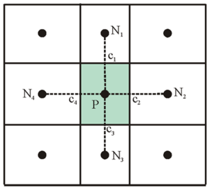
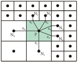
One important aspect of incompressible flow models is the location of primary variables: velocity and pressure (water level). On a staggered grid, the pressure (water level) is located at the center of cells and the u- and v-velocities are located along the faces of cells (Harlow and Welsh 1965; Patankar 1980). On a non-staggered grid, all of the primary variables are located at the center of cells. This can lead to the spatial oscillations referred to as checkerboard oscillations and model instability if the linear interpola-tion between nodes is used to determine the fluxes at cell faces. A staggered grid can more easily eliminate these oscillations when compared to a non-staggered grid; however, a non-staggered grid involves a simpler source code and can minimize the number of coefficients that must be computed and stored during a simulation because many of the terms in the equations are equal. In particular, a staggered grid is more complicated when handling the interface between coarse and fine cells where 5- or 6-face control volumes are used. Therefore, a non-staggered (collocated) grid approach is adopted for CMS-Flow with a Rhie and Chow (1983) momentum interpolation technique used to eliminate the checkerboard oscillations. Figure 3 shows the location of primary variables on the 5- and 7-point stencils (computational molecule).
Figure 3. Computational stencils and control volumes for two types of Cartesian grids: non-uniform Cartesian (left) and telescoping grid (right).
The data structure for a grid can be approached in three ways: 1) block-structured, 2) hierarchical tree, and 3) unstructured. The block-structured approach divides the domain into multiple blocks, and each block is treated as structured. The block structured approach requires a special treatment between blocks to ensure mass and momentum balance using this approach. The hierarchical tree approach is memory intensive and requires parent-child relationships and a tree traverse to determine mesh connectivity. For the unstructured approach, all cells are numbered in a 1D sequence, and tables are used to determine the connectivity of neighboring cells. Among these three approaches, the unstructured approach is the most simple and is therefore applied in CMS-Flow. Computational cells are numbered in an unstructured manner via a 1D index array. Inactive cells (permanently dry) are not included in the 1D index array to save memory and computational time. All active computational cells are numbered sequentially. It is noted that using an unstructured data approach does not limit the model from using matrix solvers designed for structured grids. For convenience with handling boundary conditions, each boundary cell has a neighboring ghost cell outside of the computational domain.
General Transport Equation
|
|
(1) |
where:
- = general scalar
- h = total water depth [m]
- = correction factor [-]
- = total flux velocity [m/s]
- = diffusion coefficient for []
- S = source/sink term which includes all remaining terms.
Note that in the case of the continuity and momentum equations, is equal to 1 and respectively. In the case of sediment and salinity transport, is equal to and , respectively. The correction factor (β) is equal to the total-load correction factor and equal to 1 for all other equations.
Spatial Discretization
A control-volume technique is used in which the governing equations are integrated over a control volume to obtain an algebraic equation that can be solved numerically. Integration of Equation (1) over a control volume yields:
|
|
(2) |
|
|
(3) |
|
|
(4) |
where
- = outward unit vector normal to cell face f [-]
- = outward cell face velocity [m/s]
- = value of at the cell centroid
- = total water depth at the cell face centroid [m]
- = interpolated total water depth at cell face f [m]
- = outward normal gradient of at cell face f:
- = interpolated diffusion coefficient for
- = area of cell P [m/s]
- = length of cell face f [m]
- = source/sink term.
In the above equations, the Gauss Divergence Theorem has been used to convert the area integral to a boundary integral. In addition, the area ingegrals have been evaluated assuming variable vary linearly within cells. The cell face velocity, , is calculated using a momentum interpolation method similar to that of Rhie and Chow (1983) and is described in Hydrodynamics of the present Chapter.
Temporal Discretization
The general transport equation is rewritten as
| (5) |
where includes all the remaining terms. For stability and efficiency, a fully implicit time-stepping scheme is used in the form
where includes all the remaining terms, such as …. For stability and efficiency, a fully implicit time-stepping scheme is used in the form
| (6) |
where is a weighting factor between 0 and 1. For , the scheme reduces to the first-order backward Euler scheme, and with , the scheme reduces to the second-order backward scheme (Ferziger and Peric 1997). The superscripts indicate the time step levels, with n+1 being the next time-step and n being the previous time-step.
Cell-face Interpolation Operator
The general formula for estimating the cell-face value is given by
| (7) |
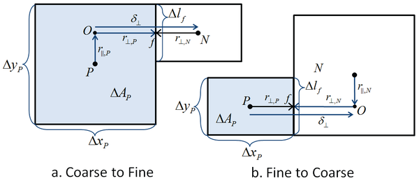
where is a linear interpolation factor, is the gradient operator in the direction parallel to face f, and is the distance from the cell center to the ghost point (O) parallel to the cell face (f) (see Figure 4).
Figure 4. Schematic showing interface interpolation: (a) coarse to fine and (b) fine to coarse.
The subscripts and indicate the components parallel and normal to the cell face. By definition, . Note that for neighboring cells without any refinement, is equal to zero and the above equation is consistent with non-refined cell faces. The linear interpolation factor is defined as
|
|
(8) |
where is the coordinate of f perpendicular to the face and is the cell dimension perpendicular to the face f.
Cell-face Gradient
A linearly exact second-order approximation for the normal gradient at cell face f is calculated using the auxiliary node concept of Ferziger and Peric (1997):
| (9) |
where the subscripts P and N refer to two neighboring cells, is the distance between cells P and N, normal to the cell face (Figure 4), and is the gradient operator in the direction parallel to face f. Ham et al. (2002) compared the auxiliary node formulation to the fully-unstructured discretization proposed by Zwart et al. (1998) for the viscous terms and found that the auxiliary node formulation is significantly more stable.
Cell-centered Gradient
The cell-centered gradient operator is calculated using the Gauss’ Divergence Theorem as
| (10) |
The equation above is second order and conservative for regular and non-uniform grids.
Reconstruction, Monotonicity, and Slope Limiters
Variables are linearly reconstructed within the cells as
| (11) |
where is the cell-average value specified at the cell centroid, is the distance vector from the cell centroid to any location within the cell, and is the cell-centered gradient. The reconstruction is second order and conservative in the sense that . The linear reconstruction is used when interpolating cell-face values (Equation 7) and calculating cell-face gradients (Equation 13). If the reconstruction satisfies the local maximum principle
| (12) |
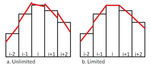
then no new extrema are created within the cell, and the solution is monotonic. Figure 5 shows two examples of linear reconstruction with and without slope limiters to ensure monotonicity.
Figure 5. Schematics showing examples of (a) non-limited and (b) limited linear reconstructions.
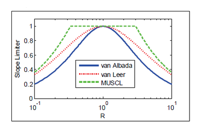
For non-telescoping grids, the slope limiter is calculated as
| (13) |
where R is the ratio between two consecutive slopes
| (14) |
Here, the second-order van Leer (1979) limiter is used because of its smoothness. Figure 6 shows a comparison of three different common limiters. The slope limiter is applied in each direction separately.
Figure 6. Comparison of three different slope limiters.
For unstructured grids the slope limiters described above are difficult to implement because of the difficulty in defining forward and backward differences. For telescoping grids the following Limited Central Difference (LCD) slope limiting procedure of Hubbard (1999) is applied:
| (15) |
where . In the procedure outlined by Hubbard (1999), a scalar limiter is then calculated as . Here, a directional limiter is applied as , which is less dissipative. Finally, the cell-centered gradient is limited as
| (16) |
where is the unlimited gradient.
Advection Schemes
Hybrid Scheme
The hybrid scheme is composed of a first-order upwind scheme and a second-order central difference scheme. The cell-face advective value is given by
| (17) |
where the subscripts D and C indicate the downstream and upstream values, and is the Peclet number at the cell face in which ,. In the hybrid scheme, when the Peclet number is larger than 2, the first-order upwind value is used; otherwise, the second-order central difference value is used.
Exponential Scheme
The exponential scheme interpolates the face value using an exact solution to the 1D steady advection-diffusion equation:
| (18) |
The exponential scheme has automatic upwinding and is stable but is usually less than second order.
Hybrid Linear/Parabolic Scheme
The Hybrid Linear/Parabolic Approximation (HLPA) scheme of Zhu (1991) may be written as
| (19) |
where the subscripts D, C, and U indicate the first downstream and first and second upstream cells, respectively. The normalized variable ) is determined based on the formulation of Jasak et al. (1999)
| (20) |
where . The HLPA scheme is second order. Choi et al. (1995) found that the HLPA scheme has similar accuracy to the third-order SMARTER (Sharp and Monotonic Algorithm for Realistic Transport Efficiently Revised) and LPPA (Linear and Piecewise-Parabolic Approximation) schemes but is simpler and more efficient (Shin and Choi 1992; Choi et al. 1995).
Source/sink Term
The source/sink term is linearized as (Patankar 1980)
| (21) |
The coefficient is required to be non-positive for stability.
Assembly of Algebraic Equations
Assembly refers to the process of combining terms to create a linear sys-tem of algebraic equations. The algebraic equation for each cell is obtained by first combining or assembling all of the terms. Then, the continuity equation is multiplied by and is subtracted from the transport equation. The resulting discretized equation for cell P is
| (22) |
where the subscript N refers to the neighboring cell sharing cell face, and are linear coefficients for and . The last term, (b) contains all the remaining terms. Applying a similar equation for all of the internal cells of a grid results in a system of algebraic equations. This set of equations are referred to as the discretized governing equations.
Implicit Relaxation
The right-hand side of the algebraic system of equations (b) generally contains deferred corrections and source terms which must be computed iteratively. This iteration loop is referred to as the outer loop, and the loop within the linear iterative solver (see Section Iterative Solvers) is referred to as the inner loop. Under-relaxation is often applied to stabilize the convergence of the outer iteration loop. Under-relaxation may be applied as in which is an under-relaxation parameter . The superscript m indicates the previous iteration, and superscript m+1 indicates the new relaxed value. A better approach is used here to introduce the under-relaxation directly in the algebraic system of equations (Majumdar 1988; Ferziger and Peric 1997) as
| (23) |
This is referred to implicit under-relaxation and has the effect of making the coefficient matrix more diagonally dominant, thus improving convergence.
Iterative Solvers
The selection of an iterative solver is one key issue concerning the overall per-formance of the model. CMS has three iteration solvers available and they are described in more detail below: 1) GMRES variation, 2) BiCGStab, and 3) Gauss-Seidel. The default iterative solver for CMS is a variation of the GMRES (Generalized Minimum RESidual) method (Saad 1993) and is used to solve the algebraic equations. The original GMRES method (Saad and Schultz 1986) utilizes the Arnoldi process to reduce the coefficient matrix to the Hessenburg form and minimizes the norm of the residual vector over a Krylov subspace at each iterative step. The variation of the GMRES method recommended by Saad (1993) allows changes in preconditioning at every iteration step. An Incomplete LU Factorization (ILUT; Saad, 1994) is used as the preconditioner to speed-up convergence. The GMRES solver is applicable to symmetric and non-symmetric matrices and leads to the smallest residual for a fixed number of iterations. However, the memory requirements and computational costs become increasingly expensive for larger systems.
The BiCGStab (BiConjugate Gradient Stabilized) iterative solver is also a Krylov subspace solver and is applicable to symmetric and non-symmetrix matrices (Saad 1996). BiCGStab also uses ILUT as a preconditioner (Saad 1994). The BiCGStab method can be viewed as a combination of the standard Biconjugate Gradient solver where each iterative step is followed by a restarted GMRES iterative step. One advantage of the BiCGStab iterative solver is that the memory requirements are constant for each iteration and there are less computational costs when compared to the GMRES method (for less than four iterations).
The SIP (Strongly Implicit Procedure) iterative solver uses an Incomplete Lower Upper decomposition, which approximates the exact Lower Upper decomposition (Stone 1968). The method is specifically designed for algebraic systems of equations derived from partial differential equations. The implementation here is for a 5-point stencil and, therefore, only applies to nontelescoping grids.
The ICCG (Incomplete Cholesky preconditioned Conjugate Gradient) iterative solver is applicable to symmetric matrices such as the pressure correction equation (Ferziger and Peric 2002). The implementation here is also for a 5-point stencil and, therefore, can only be applied to nontelescoping grids.
The simplest iterative solver implemented in CMS is the point-implict Gauss-Seidel solver. This method may be applied in CMS with or without Succesive-Over-Relaxation to speed-up convergence (Patankar 1980). Even though the Gauss-Seidel method requires more iterations for convergence, the overall efficiency may be higher than the GMRES and BiCGStab because each itera-tion is computationally inexpensive and the code is parallelized. However, the GMRES and BiCGStab methods are more robust and perform better for large time-steps.
Convergence and Time-Stepping
During the iterative solution process, error is calculated and used to de-termine if a solution has converged, diverged, or stalled at an error below a set tolerance threshold. Anestimate of the error in solving the general algebraic equation is given by
| (24) |
The -norm of the residual is given by
| (25) |
Since this value depends on the total number of cells, the final statistic (referred to as the residual) that is used for estimating the model convergence is obtained by dividing the l2norm by the square root of the number of cells:
| (26) |
where Nc is the number of computational cells. Simply stated, Rm is referred to as the normalized residual error, and the superscript refers to the iteration number. Also, Rm is calculated for each variable that is solved at each iteration step of the solution process. Each equation has default maximum tolerances for determining if the solution has converged, diverged, or stalled. The maximum number of iterations that is imposed is set equal to M. A minimum of five iterations is required for the hydrodynamic equations, and a minimum of M/2 iterations is required for the sediment transport equations. Table 1 lists the default criteria to determine whether the iterative solution procedure has converged, requires a reduced time-step, or has diverged.
| Current velocity, m/s |
If Rm < 1x10⁻⁷ | If RM > 1.0x10⁻² or |Ui| > 10 |
If RM > 1.0x10⁻³ |
| Pressure- correction, m2/s2 |
If RM < 1x10⁻⁸ | If RM > 1.0x10⁻³ or |p| >50 |
If RM>1.0x10⁻⁴ |
| Total-load concentration, kg/m3 |
If RM<1x10⁻⁸ | If Rm>1.0x10⁻³ or Ctk<0 |
None |
| Salinity, ppt | If Rm<1x10⁻⁶ | If Csal < 0 | None |
For the implicit model, the time steps for the hydrodynamics, sediment and salinity transport are the same in order to avoid mass conservation problems and for simplicity. If any of the time step reduction criteria are met, then the time step is reduced by half and a minimum number of 3 time steps are calculated at the newly reduced time step. If the last time step converged properly, then the time step is increased. The maximum time step allowed is equal to the user-specified initial time step.
Ramp Period
For most coastal applications, the model is initialized from a “cold start”, which means that the water level and current velocities are initially set to zero. The ramp period allows the model to slowly transition from the ini-tial condition without “shocking” the system. In CMS, the ramp function is defined as
| (27) |
where t is the simulation time and is the ramp duration. The ramp function provides a smooth function for transitioning from the initial conditions and is plotted in Figure 7.
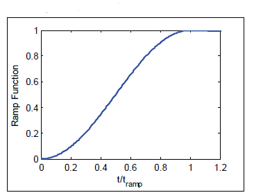
Figure 7. Ramp function used in CMS
The ramp function is applied to the model forcing conditions, including the wave forcing , surface wind , sediment concentration capacity , and significant wave height , by direct multiplication of these parameters by the ramp function at each time step during the ramp period. Boundary conditions in CMS are specified without consideration of this ramp period; therefore, the boundary conditions are also slowly transitioned from the initial condition by direct multiplication of the boundary conditions by the ramp function at each time step during the ramp period.
References
- Buttolph, A. M., C. W. Reed, N. C. Kraus, N. Ono, M. Larson, B. Camenen, H. Hanson, T. Wamsley, and A. K. Zundel. 2006. Two-dimensional depth-averaged circulation model CMS-M2D: Version 3.0, Report 2: Sediment transport and morphology change. ERDC/CHL TR-06-9. Vicksburg, MS: US Army Engineer Research and Development Center.
- Choi, S. K., H .Y. Nam, and M. Cho. 1995. A comparison of higher-order bounded convection schemes. Computational Methods in Applied Mechanics and Engineering (121):281-301.
- Ferziger, J. H., and M. Peric. 1997. Computational methods for fluid dynamics. Berlin/New York: Springer-Verlag.
- Harlow, F. H., and J. E. Welch. 1965. Numerical calculation of time-dependent viscous incompressible flow of fluid with free surface. Physics of Fluids (8): 2182.
- Hubbard, M. E. 1999. Multidimensional slope limiters for MUSCL-type finite volume schemes on unstructured grids. Journal of Computational Physics (155):54–74.
- Jasak, H., H. G., Weller, and A. D. Gosman. 1999. High resolution NVD differencing scheme for arbitrarily unstructured meshes. International Journal of Numerical Methods for Fluids (31):431–449.
- Majumdar, S. 1988. Role of underrelaxation in employing momentum interpolation practice for calculation of flow with non-staggered grids. Numerical Heat Transfer (13):125–132.
- Patankar, S. V. 1980. Numerical heat transfer and fluid flow. New York: Hemisphere,
- Rhie, T. M., and A. Chow. 1983. Numerical study of the turbulent flow past an isolated airfoil with trailing-edge separation. AIAA Journal (21):1525–1532.
- Shin, J. K., and Y. D. Choi. 1992. Study on the improvement of the convective differencing scheme for the high-accuracy and stable resolution of the numerical solution [in Korean]. Transactions KSME 16(6):1179–1194.
- Stone, H. L. 1968. Iterative solution of implicit approximations of multidimensional partial differential equations. SIAM Journal of Numerical Analysis 5(3):530–538.
- van Doormaal, J. P. and Raithby, G. D. 1984. Enhancements of the SIMPLE method for predicting incompressible fluid flows. Numerical Heat Transfer (7): 147–163.
- van Albada, G. D., B. van Leer, and W. W. Roberts. 1982. A comparative study of computational methods in cosmic gas dynamics. Astronomy and Astrophysics (108):76–84.
- van Leer, B. 1979. Toward the ultimate conservative difference scheme. V. A second order sequel to Godunov method. Journal of Compuational Physics (32):101–136.
- Wu, W., A. Sánchez, and M. Zhang. 2011. An implicit 2-D shallow water flow model on an unstructured quadtree rectangular grid. Journal of Coastal Research, Special Issue (59):15–26.
- Zwart, P. J., G. D., Raithby, and M. J. Raw. 1998. An integrated space-time finite volume method for moving boundary problems. Numerical Heat Transfer (B34):257.
