User Guide 004: Difference between revisions
No edit summary |
No edit summary |
||
| (One intermediate revision by the same user not shown) | |||
| Line 236: | Line 236: | ||
Figure 2-36. CMS-Flow Wind tab in the CMS-Flow Model Control window in SM 11.1. | Figure 2-36. CMS-Flow Wind tab in the CMS-Flow Model Control window in SM 11.1. | ||
Table 2-34. CMS cards used for spatially constant wind forcing. | |||
{|class="wikitable" | |||
|- | |||
!Input | |||
!Format | |||
!Notes | |||
|- | |||
|Wind | |||
Time Series | |||
Curve | |||
|[card=WIND_INPUT_CURVE] | |||
[name=WindFile, type=char, | |||
default=MPFile] | |||
[name=WindPath, type=char, default= | |||
”PROPERTIES/Model Params/WindCurve”] | |||
|File name and path of the spatially constant wind time series. | |||
|} | |||
=Spatially Variable Wind and Atmospheric Pressure= | =Spatially Variable Wind and Atmospheric Pressure= | ||
| Line 252: | Line 268: | ||
This file format is equivalent to the ADCIRC fort.22 format with NWS=6. The winds and atmospheric pressure are specified on a rectangular grid at constant temporal intervals. The wind grid is assumed to be in the same horizontal coordinate system as the CMS grid. The wind data is spatially interpolated using an inverse distance method and temporally interpolated using linear interpolation. The grid is assumed to vary from North to South and West to East so that north-west corner is the grid origin. The spatial extents of the wind/pressure grid must be consistent with the flow grid. The wind file is written from West to East starting at the North-West Corner. The file is read in free format. An example of section of a single ASCII Wind File is shown below: | This file format is equivalent to the ADCIRC fort.22 format with NWS=6. The winds and atmospheric pressure are specified on a rectangular grid at constant temporal intervals. The wind grid is assumed to be in the same horizontal coordinate system as the CMS grid. The wind data is spatially interpolated using an inverse distance method and temporally interpolated using linear interpolation. The grid is assumed to vary from North to South and West to East so that north-west corner is the grid origin. The spatial extents of the wind/pressure grid must be consistent with the flow grid. The wind file is written from West to East starting at the North-West Corner. The file is read in free format. An example of section of a single ASCII Wind File is shown below: | ||
Example 2-18. Excerpt of a Wind and Atmospheric Pressure File: | |||
---- | |||
7.5835 1.2324 0.00 | |||
7.5835 1.2324 0.00 | |||
7.5835 1.2324 0.00 | |||
... | |||
---- | |||
Example 2-19. FORTRAN code used to read the file is shown below: | |||
---- | |||
!For each wind snap shot | |||
do i=1,nwindi | |||
do j=1,nwindj | |||
read(wunit,*,end=444) wndspdx(i,j),wndspdy(i,j),atmpres(i,j) | |||
enddo !j | |||
enddo !i | |||
---- | |||
Example 2 20. Specifying a wind and atmospheric pressure file and parameters. | |||
---- | |||
WIND_PRESSURE_SINGLE_FILE “wind.dat” | |||
WIND_PRESSURE_GRID_PARAM 201 201 50000.0 -50000.0 500.0 500.0 | |||
WIND_PRESSURE_TIME_INCREMENT 360000.0 !seconds | |||
---- | |||
A description of the cards related to winds and atmospheric pressure are described in the table below. | A description of the cards related to winds and atmospheric pressure are described in the table below. | ||
Table 2-35. CMS-Flow cards related to winds and atmospheric pressure | |||
{|class="wikitable" | |||
|- | |||
!Input | |||
!Format | |||
!Notes | |||
|- | |||
|Wind Pressure Single File | |||
|[card=WIND_PRESSURE_SINGLE_FILE] | |||
[name=WindFile, type=char] | |||
|File name and path of the spatially constant wind time series. | |||
|- | |||
|Wind Pressure XY file | |||
|[card=WIND_PRESSURE_XY_FILE] | |||
[name=windlocfile, type=char] | |||
|Name of coordinate file (*.xy). | |||
|- | |||
|Wind Pressure Time Increment | |||
|[card=WIND_PRESSURE_TIME_INCREMENT] | |||
[name=wtiminc, type=float, | |||
units=sec] | |||
|Specifies the the met file time series increment (SwTimeInc) in seconds | |||
|- | |||
|Wind Pressure Grid Parameters | |||
|[card=WIND_PRESSURE_GRID_PARAM] | |||
[name=nwindi, type=int, range= >0] | |||
[name=nwindj, type=int, range= >0] | |||
[name=wlatmax, type=float] | |||
[name=wlonmin, type=float] | |||
[name=wlatinc, type=int, range= >0] | |||
[name=wloninc, type=int, range= >0] | |||
|Specifies the grid parameters for the wind and pressure file. | |||
nwindi = number of latitude or y-coordinate. | |||
nwindj = number of longitude or x-coordinate | |||
nwindj = maximum latitude (decimal deg) or y-coordinate of data in met file (< 0 south of the equator). | |||
wlatmax = maximum latitude(decimal deg) or x-coordinateof data in the met file (< 0 west of Greenwich meridian). | |||
wlonmin = minimum longitude (decimal deg) or x-coordinateof data in the met file (< 0 west of Greenwich meridian). | |||
wlatinc = latitude or y-coordinate increment (decimal deg) of data in the met file (must be > 0). | |||
wloninc = longitude or x-coordinate increment (decimal deg) of data in the met file (must be > 0). | |||
|} | |||
=Notes= | =Notes= | ||
Latest revision as of 15:52, 7 May 2015
Wall Friction
Two boundary conditions are available for the tangential flow at closed boundaries:
- 1. Free-slip: No tangential shear stress (no wall friction);
- 2. Partial-slip: Tangential shear stress (wall friction) calculated based on the log law.
Wall friction enhances the flow drag perpendicular to any closed bounda-ry. Assuming a log law for a rough wall, the partial-slip tangential shear stress is given by
| (2-5) |
where is the magnitude of the wall parallel current velocity, and cwall is the wall friction coefficient equal to
| (2-6) |
Here, y0 is the roughness length of the wall and is assumed to be equal to that of the bed (i.e., y0 = z0 ). The distance from the wall to the cell center is yp .
Table 2-31. SMS Cards related to the wall friction
| Input | Format | Notes |
|---|---|---|
| Wall Friction | [card=USE_WALL_FRICTION_TERMS]
[name=wallfric, type=char, options=(ON,OFF), default=OFF] |
Turns on or off wall friction |
Example 2-16. Specifying the wall friction.
USE_WALL_FRICTION_TERMS ON !ON | {OFF}
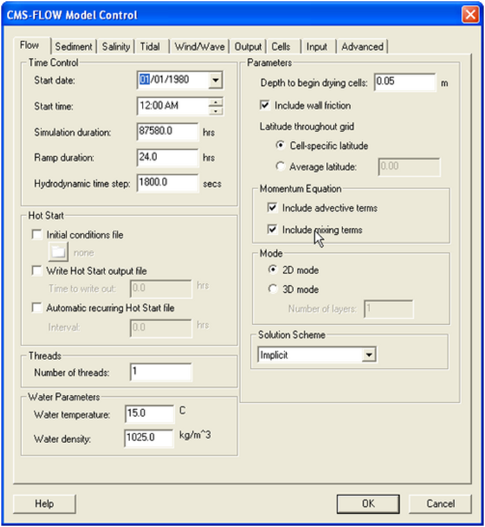
The wall friction may be turned ON or OFF in the Flow tab of the CMS-Flow Model Control window (see Figure 2-30). The default in SMS is for the wall friction to be ON. Table 2-31 shows the CMS card used activating the wall friction.
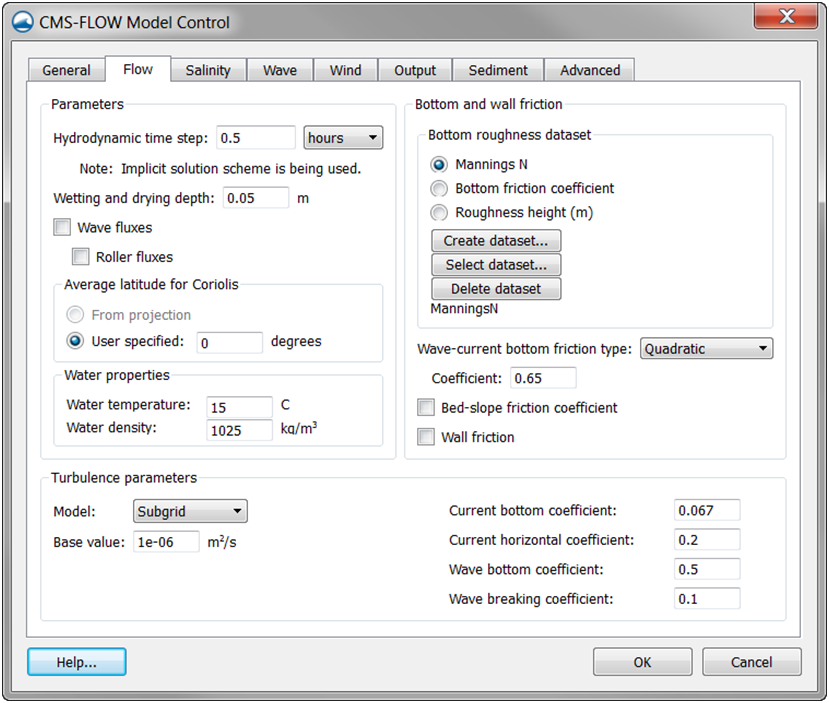
Figure 2-30. Wall friction specification in the CMS-Flow Model Control window of SMS 11.0.
Figure 2-31. Wall friction specification in the CMS-Flow Model Control window of SMS 11.1.
Eddy Viscosity
The term eddy viscosity arises from the fact that small-scale vortices or eddies on the order of the grid cell size are not resolved, and only the large-scale flow is simulated. The eddy viscosity is intended to simulate the dissipation of energy at smaller scales than the model can simulate. In the nearshore environment, large mixing or turbulence occurs due to waves, wind, bottom shear, and strong horizontal gradients. Therefore, the eddy viscosity is an important parameter which can have a large influence on the calculated flow field and resulting sediment transport. In CMS-Flow, the total eddy viscosity ( ) is equal to the sum of three parts: 1) a base value ( ); 2) the current-related eddy viscosity ( ); and 3) the wave-related eddy viscosity ( ) defined as follows:
| (2-7) |
The base value ( ) is approximately equal to the kinematic viscosity (~1.81×10⁻⁶ m2/s) but may be changed by user. The other two components ( and ) are described in the sections below.
There are four algebraic models for the current-related eddy viscosity: 1) Falconer Equation, 2) depth-averaged parabolic, 3) subgrid, and 4) mix-ing-length. The default turbulence model is the subgrid model but may be changed by the user. The wave-related eddy viscosity consists of two components representing turbulence generated at the bed due to oscillatory flow, and at the surface due to wave breaking.
In SMS 11.0 all of the eddy viscosity options and parameters are entered via Advanced Cards and only the option is given to turn On or Off the mixing terms (see Figure 2-32).
Figure 2-32. Toggle for turning On and Off the mixing terms in the SMS 11.0 interface
Figure 2-33. Eddy viscosity parameter specifiecation within the Flow tab of the CMS-Flow Model Control window in SMS 11.1
A description of the CMS-Flow Cards related to eddy viscosity is shown, below, in the table below.
Table 2-32. CMS card used to set turbulence model and eddy viscosity terms
Eddy Viscosity Wave| Input | Format | Notes |
|---|---|---|
| Mixing Terms | [card=USE_MIXING_TERMS]
[name=mturbul, type=char, options=(ON,OFF), default=ON] |
Deprecated. Turns On and Off the mixing terms in the momentum and transport equations. |
| Turbulence Model | [card=TURBULENCE_MODEL]
[name=mturbul, type=char, options=(SUBGRID,FALCONER, PARABOLIC,MIXING-LENGTH, default=SUBGRID] |
Specifies the turbulence model used. For details on the different turbulence models see section Eddy Viscosity. |
| Eddy
Viscosity Constant |
[card=EDDY_VISCOSITY_CONSTANT]
[name=cviscon, type=float, default=1.0E-6, range=(cviscon>=0.0)] |
Constant contribution or base value of eddy viscosity |
| Eddy
Viscosity Bottom |
[card=EDDY_VISCOSITY_BOTTOM]
[name=cviscon, type=float, default=0.0667, range=0.02-0.1] |
Coefficient related to the contribution to eddy viscosity from the bottom shear |
| Eddy
Viscosity Horizontal |
[card=EDDY_VISCOSITY_HORIZONTAL]
[name=cvishor, type=float, default=0.2, range= 0.1-0.2] |
Coefficient related to the contribution to eddy viscosity from horizontal velocity gradients |
| [card=EDDY_VISCOSITY_WAVE]
[name=cviswav, type=float, default=0.5, range=0.2-1.0] |
Coefficient related to the wave bottom friction contribution to eddy viscosity | |
| Eddy
Viscosity Breaking |
[card=EDDY_VISCOSITY_BREAKING]
[name=cviswavbrk, type=float, default=0.05, range=0.05-0.1] |
Coefficient related to the wave breaking contribution to eddy viscosity |
Notes:
- 1. The eddy viscosity can be calibrated by looking at several features of the flow. Increasing the eddy viscosity
- a. Increases the width of the longshore current.
- b. Increases the spread of the ebb and flood tidal jet currents.
- c. Decreases the offshore extent of the ebb jet current.
- d. Smoothes out small gyres and recirculation zones.
- 2. The eddy viscosity affects the sediment mixing since the sediment mixing coefficient is calculated as the eddy viscosity divided by the Schmidt number.
- 3. The eddy viscosity can be used to dampen out model (by increasing its value). However, this should be done with caution and is only recom-mended as a last resort. Usually, model instabilities are linked to bathymetry or boundary problems and can be resolved by other means.
Wave Mass Flux
The wave mass (or volume) flux has two contributions; one due to Stokes drift (mass transport above the trough level) and the second due to the surface roller. The Stokes drift component is due to the oscillatory wave motion and is always present. The surface roller flux is due to the breaking waves and is only present in the surf zone. The mean wave mass flux velocity, or simply the mass flux velocity for short, is defined as the mean wave volume flux divided by the local water depth and is approximated here as (Phillips 1977; Ruessink et al. 2001; Svendsen 2006)
| (2-8) |
where
- Ew = wave energy = [N/m]
- Hs = significant wave height [m]
- Esr = surface roller energy density [N/m]
- wi = wave unit vector (cos , sin ) [-]
- c = wave speed [m/s]
- = mean wave direction, [rad]
The first component is due to the wave energy (Ew is the Stokes velocity), while the second component is due to the surface roller (Esr is only present in the surfzone). Therefore the total flux velocity Vi may be written as
| (2-9) |
where Ui is the depth-averaged current velocity. Turning on the Wave Mass Flux activates the wave flux velocity. This velocity always includes the Stokes velocity. However, the surface roller component is optional and can be turned on separately, but only if the wave mass flux is on and the surface roller model is also activated. The table below describes the CMS cards used to activate the wave mass flux and surface roller mass flux.
Table 2-33. CMS card used to turn on or off the wave volume flux velocities
| Input | Format | Notes |
|---|---|---|
| Wave
Mass Flux |
[card=WAVE_MASS_FLUX]
[name=WaveFlux, type=char, options=(ON,OFF), default=OFF] |
Turns on and off the wave volume flux velocities |
| Roller
Mass Flux |
[card=ROLLER_MASS_FLUX]
[name=RolFlux, type=char, options=(ON,OFF), default=OFF] |
Turns on or off the contribution to the wave volume flux velocities due to the surface roller in the surf zone. Only used if surface roller model is turned on. |
Example 2-17. Wave mass flux specification.
WAVE_MASS_FLUX ON !{OFF} | ON ROLLER_MASS_FLUX ON !{OFF} | ON, Only applicable if wave flux is on
As mentioned by Svendsen (2006), the Stokes drift component of the wave mass flux from linear wave theory is expected to be an overestimation in the surf zone since nonlinear waves are less “bulky” and therefore transport less mass. For this reason, it can be argued in favor of neglecting the surface roller component in the surf zone to compensate for the overestimation of the Stokes velocity. By default, the wave mass flux is off.
Notes
- It is recommended to use the wave mass flux without the roller component. This usually leads to the best results.
Wind and Atmospheric Pressure Forcing
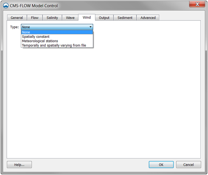
The wind and atmospheric pressure forcing are specified in the Wind tab of the CMS-Flow Model Control Window (see figure below). There are four main options for the wind and atmospheric pressure forcing
- 1. None
- 2. Spatially constant time-series
- 3. Meteorological Stations
- 4. Temporally and spatially varying
Figure 2-34. CMS-Flow Wind tab in the CMS-Flow Model Control window in SM 11.1.
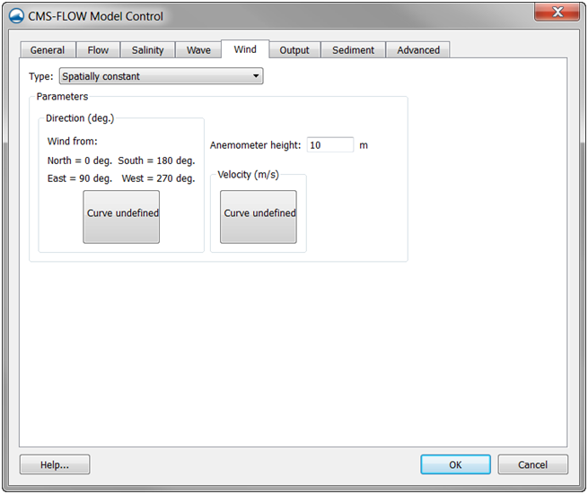
Spatially Constant Wind Time series
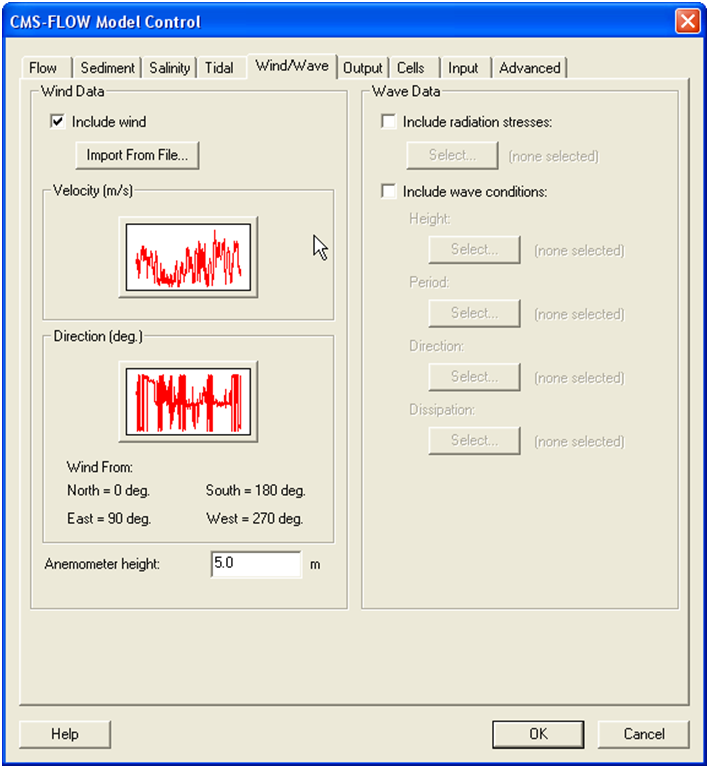
Spatially constant wind is specified in the Wind/Wave tab of the CMS-Flow Model Control window (see Figure 2-35).
Figure 2-35. CMS-Flow Wind/Wave tab in the CMS-Flow Model Control window in SM 11.0.
Figure 2-36. CMS-Flow Wind tab in the CMS-Flow Model Control window in SM 11.1.
Table 2-34. CMS cards used for spatially constant wind forcing.
| Input | Format | Notes |
|---|---|---|
| Wind
Time Series Curve |
[card=WIND_INPUT_CURVE]
[name=WindFile, type=char, default=MPFile] [name=WindPath, type=char, default= ”PROPERTIES/Model Params/WindCurve”] |
File name and path of the spatially constant wind time series. |
Spatially Variable Wind and Atmospheric Pressure
CMS-Flow V4.0 (and higher) has the option to use spatially variable wind and atmospheric pressure forcing. Currently, this feature is specified in the advanced card section. There are currently two input options for spatially variable winds and atmospheric pressure: (1) Single ASCII Wind/Pressure File and (2) Multiple Oceanweather Files. These input formats and their cards are described in the following sections. When using spatially variable winds and atmospheric pressure it is good to keep in mind the following notes.
Notes
- 1.Interpolation File: When using spatially variable winds CMS will out-put a file named Intpcoef_wndfl.bin. This file contains the coefficients used to interpolate the winds and atmospheric pressure to the CMS-Flow grid. If the same flow and wind grids are run, the model will automatically detect the interpolation file and read in the coefficients instead of calculating them. If the either grid is changed in size, the model will automatically detect this and recalculate the coefficients. However, if the grids are changed but stay the same size, the model will not be able to detect that they have changed. Therefore, whenever any changes are made to the flow or wind grids, it is best to delete the prior interpolation file.
- 2. Ramp Period: During the ramp period, the ramp is applied to both the wind shear stresses and spatial variations of the atmospheric pressure.
Wind and Atmospheric Pressure File
This file format is equivalent to the ADCIRC fort.22 format with NWS=6. The winds and atmospheric pressure are specified on a rectangular grid at constant temporal intervals. The wind grid is assumed to be in the same horizontal coordinate system as the CMS grid. The wind data is spatially interpolated using an inverse distance method and temporally interpolated using linear interpolation. The grid is assumed to vary from North to South and West to East so that north-west corner is the grid origin. The spatial extents of the wind/pressure grid must be consistent with the flow grid. The wind file is written from West to East starting at the North-West Corner. The file is read in free format. An example of section of a single ASCII Wind File is shown below:
Example 2-18. Excerpt of a Wind and Atmospheric Pressure File:
7.5835 1.2324 0.00 7.5835 1.2324 0.00 7.5835 1.2324 0.00 ...
Example 2-19. FORTRAN code used to read the file is shown below:
!For each wind snap shot do i=1,nwindi
 do j=1,nwindj
   read(wunit,*,end=444) wndspdx(i,j),wndspdy(i,j),atmpres(i,j)
 enddo !j
enddo !i
Example 2 20. Specifying a wind and atmospheric pressure file and parameters.
WIND_PRESSURE_SINGLE_FILE “wind.dat” WIND_PRESSURE_GRID_PARAM 201 201 50000.0 -50000.0 500.0 500.0 WIND_PRESSURE_TIME_INCREMENT 360000.0 !seconds
A description of the cards related to winds and atmospheric pressure are described in the table below.
Table 2-35. CMS-Flow cards related to winds and atmospheric pressure
| Input | Format | Notes |
|---|---|---|
| Wind Pressure Single File | [card=WIND_PRESSURE_SINGLE_FILE]
[name=WindFile, type=char] |
File name and path of the spatially constant wind time series. |
| Wind Pressure XY file | [card=WIND_PRESSURE_XY_FILE]
[name=windlocfile, type=char] |
Name of coordinate file (*.xy). |
| Wind Pressure Time Increment | [card=WIND_PRESSURE_TIME_INCREMENT]
[name=wtiminc, type=float, units=sec] |
Specifies the the met file time series increment (SwTimeInc) in seconds |
| Wind Pressure Grid Parameters | [card=WIND_PRESSURE_GRID_PARAM]
[name=nwindi, type=int, range= >0] [name=nwindj, type=int, range= >0] [name=wlatmax, type=float] [name=wlonmin, type=float] [name=wlatinc, type=int, range= >0] [name=wloninc, type=int, range= >0] |
Specifies the grid parameters for the wind and pressure file.
nwindi = number of latitude or y-coordinate. nwindj = number of longitude or x-coordinate nwindj = maximum latitude (decimal deg) or y-coordinate of data in met file (< 0 south of the equator). wlatmax = maximum latitude(decimal deg) or x-coordinateof data in the met file (< 0 west of Greenwich meridian). wlonmin = minimum longitude (decimal deg) or x-coordinateof data in the met file (< 0 west of Greenwich meridian). wlatinc = latitude or y-coordinate increment (decimal deg) of data in the met file (must be > 0). wloninc = longitude or x-coordinate increment (decimal deg) of data in the met file (must be > 0). |
Notes
- 1. The wind is assumed to start at the start of the CMS simulation.
- 2. The wind grid is assumed to be in the same horizontal coordinate sys-tem as the CMS grid.
- 3. The wind velocities must be in m/s and the atmospheric pressure in Pa.
- 4. If no atmospheric pressure data is available, a constant value may be specified. Since only the gradient of the atmospheric pressure is used in forcing the model, a constant atmospheric pressure is equivalent to no atmospheric pressure forcing.


![{\displaystyle c_{wall}={\big [}{\frac {\kappa }{ln(y_{p}/y_{0}))}}{\big ]}^{2}}](https://en.wikipedia.org/api/rest_v1/media/math/render/svg/7aa32501fe28a8915a20dcaf21a0ac1b53db25cb)

