User Guide 006: Difference between revisions
No edit summary |
No edit summary |
||
| (9 intermediate revisions by the same user not shown) | |||
| Line 1: | Line 1: | ||
[[File:fig_2-47.png]] | |||
Figure 2-47. CMS-Flow Boundary Conditions Window in SMS 11.1 | |||
=Wall Boundary= | |||
Flux Boundary | The wall boundary condition is a closed boundary and is applied at any cell face between wet and dry cells. Any unassigned boundary cells at the edge of the model domain are assumed to be closed and are assigned a wall boundary. A zero normal flux to the boundary is applied at closed boundaries. Two boundary conditions are available for the tangential flow | ||
The flux boundary condition is typically applied to the upstream end of a river or stream and is specified as either a constant or time-series of total water volume flux. In a 2DH model, the total volume flux needs to be | |||
(2 12 | : 1. Free-slip: No tangential shear stress (wall friction) | ||
: 2. Partial-slip: Tangential shear stress (wall friction) calculated based on the log-law | |||
Assuming a log-law for a rough wall, the partial-slip tangential shear stress is given by | |||
{{Equation|<math>\tau_{wall} = \rho c_{wall}U^2 _\Box</math>|2-10}} | |||
where <math>U_\Box</math> is the magnitude of the wall parallel current velocity and c<sub>wall</sub> is the wall friction coefficient equal to | |||
{{Equation|<math>c_{wall} = \left[\frac{\kappa}{ln(y_p /y_0)-1} \right]^2</math>|2-11}} | |||
Here y<sub>0</sub> is the roughness length of the wall and is assumed to be equal to that of the bed (i.e. y<sub>0</sub> = z<sub>0</sub> ). y<sub>p</sub>is the distance from the wall to the cell center. | |||
=Notes= | |||
:• When SMS generates a new grid, cellstrings are automatically generated along all boundaries. The default boundary type is the wall boundary. It is recommended to delete all boundary cellstrings which are not open boundary conditions, since the wall boundary conditions are automatically assigned within the model. Deleting the cellstrings avoids confusion when assigning the boundary con-ditions. | |||
:• Since the wall boundary is a closed boundary and all unassigned boundaries are treated as closed, the wall boundary cellstring in-formation does not need to written to the CMS-Flow Card File. | |||
=Flux Boundary= | |||
The flux boundary condition is typically applied to the upstream end of a river or stream and is specified as either a constant or time-series of total water volume flux. In a 2DH model, the total volume flux needs to be distributed across the boundary in order to estimate the depth-averaged velocities. This is done using a conveyance approach in which the current velocity is assumed to be related to the local flow depth ''h'' and Manning’s ''n'' as (i.e. <math>U \propto h^r / n</math> ). Here ''r'' is an empirical conveyance coefficient equal to approximately 2/3 for uniform flow. The smaller the value the more uniform the current velocities are across the flux boundary. The water volume flux, qi , at each boundary cell ''i'' is calculated as | |||
{{Equation|<math> \overrightarrow{q}_i = h \overrightarrow{U}_i = \frac{f_{Ramp}Q} {\left| \Sigma_i (\hat{e}\cdot \hat{n}) \frac{h_i ^{r+1}}{n_i} \Delta l_i \right|} \frac{h_i ^{r+1}}{n_i} \hat{e} </math>|2-12}} | |||
where | where | ||
i = subscript indicating a boundary cell | :i = subscript indicating a boundary cell | ||
: <math>\overrightarrow{q}_i</math>= volume discharge at boundary cell i per unit width [m<sup>2</sup>/s] | |||
: <math>\hat{e}</math> = unit vector for inflow direction = (sin <math>sin \phi , cos \phi</math>) | |||
: <math>\phi</math>= inflow direction measured clockwise from North [deg] | |||
: <math>\hat{n}</math>= boundary face unit vector (positive outward) | |||
:Q = total volume flux across the boundary [m<sup>3</sup>/s] | |||
:n = Manning’s coefficient [s/m<sup>1/3</sup>] | |||
:r =empirical constant equal to approximately 2/3 | |||
: <math>\Delta l</math> =cell width in the transverse direction to flow [m] | |||
: f<sub>Ramp</sub> = ramp function [-] | |||
The total volume flux is positive into the computational domain. Since it is not always possible to orient all flux boundaries to be normal to the flux boundaries, the option is given to specify an inflow direction <math>\phi</math> . The angle is specified in degrees clockwise from true North. If the angle is not specified, then the inflow angle is assumed to be normal to the boundary. The total volume flux is conserved independently of the inflow direction. | |||
As mentioned above, the total water volume flux Q<sub>B</sub> may be specified as a constant value or a single time-series curve. A description of the CMS-Flow cards used to specify the flux boundary condition information is provided in the table below. | |||
Table 2-42. CMS-Flow cards related to the flux boundary condition. | |||
{|class="wikitable" | |||
|- | |||
!Input | |||
!Format | |||
!Notes | |||
|- | |||
|Flux boundary | |||
|[card=QDRIVER_CELLSTRING] | |||
[name=Qfile, type=char, | |||
default=none] | |||
[name=Qpath, type=char, | |||
default=none] | |||
|Specifies the Boundary ID File and Path (if necessary). Outdated in CMS V4.1 and newer. Has been replaced by block structure format. | |||
|} | |||
Example 1: Single line flux boundary specification | |||
---- | |||
QDRIVER_CELLSTRING "Flow_mp.h5" "PROPERTIES/Model Params/Boundary" | |||
---- | |||
=Step-by-Step Flux Boundary Specification in SMS= | |||
The flow rate boundary condition specifies a time series of water fluxes in units of m<sup>3</sup>/s per cell. To assign a flux BC in SMS | |||
:1. If not already created by SMS, create the cellstring at the flux boundary (see section ''Creating and Deleting Cell Strings in SMS'' for details). | |||
:2. Select the cellstring (see section ''Selecting a Cellstring'' for details) | |||
:3. Open the ''CMS-Flow Boundary Conditions Window'' (see section ''Assigning a Boundary Condition'' for details). | |||
:4. Enter a time series of total flux values on and select ''OK'' button. | |||
:5. Save the SMS project File (*.sms) or ''CMS-Flow Simulation File'' (*.cmcards). | |||
Total flow rate specified is divided between the total number of cells in the cellstring with each assigned a portion of the total flux as function of the local water depth and bottom friction. | Total flow rate specified is divided between the total number of cells in the cellstring with each assigned a portion of the total flux as function of the local water depth and bottom friction. | ||
Notes: | =Notes= | ||
• The flux boundary type may ONLY be specified along cellstrings which are straight (i.e. the cellstring may not wrap around corners). | |||
• Cellstrings have to be at least three cells long. | :• The flux boundary type may ONLY be specified along cellstrings which are straight (i.e. the cellstring may not wrap around corners). | ||
• Positive fluxes are directed inward and negative fluxes are directed outward. By default the inflow/outflow angles are assumed to be normal to the boundary. The angle may be changed using the ad-vanced block structure described in the following section. | |||
• If the flux data file name and path are not specified, then they are assumed to be the same as for cellstring. | :• Cellstrings have to be at least three cells long. | ||
:• Positive fluxes are directed inward and negative fluxes are directed outward. By default the inflow/outflow angles are assumed to be normal to the boundary. The angle may be changed using the ad-vanced block structure described in the following section. | |||
:• If the flux data file name and path are not specified, then they are assumed to be the same as for cellstring. | |||
=Water Level Boundaries= | |||
The water level at a boundary can be specified as | |||
:1. Constant value | |||
:1. Single time-series curve | |||
:2. Cell-specific time-series curves (i.e. one time-series for each boundary cell) | |||
:3. Tidal constituents | |||
:4. Harmonic constituents | |||
:5. Extracted values from a parent grid simulation (nesting) | |||
:6. Tidal database | |||
The general formula for the boundary water surface elevation is given by | The general formula for the boundary water surface elevation is given by | ||
{{Equation|<math>\bar{\eta}_B = f_{Ramp} (\bar{\eta}_E + \Delta \bar{\eta} +\bar{\eta}_C + \bar{\eta}_G) + (1 - f_{Ramp}) \bar{\eta}_0</math>|2-13}} | |||
where | where | ||
The external water surface elevation may be spatially and temporally con-stant or variable. When a time series is specified, the values are interpolated using piecewise Lagrangian polynomials. By default, second order interpolation is used, but can be changed by the user. The water surface elevation offset | : <math>\bar{\eta}_B</math> = boundary water surface elevation [m] | ||
: <math>\bar{\eta}_E</math> = external boundary water surface elevation [m] | |||
: <math>\Delta\bar{\eta}</math>= water surface elevation offset [m] | |||
: <math>\bar{\eta}_0</math> = initial boundary water surface elevation [m] | |||
: <math>\bar{\eta}_C</math> = correction to the boundary water surface elevation which is a function of the wind and wave forcing [m] | |||
: <math>\bar{\eta}_G</math>= water surface elevation component derived from user speci-fied gradients [m] | |||
: f<sub>Ramp</sub>= ramp function [-] | |||
The external water surface elevation may be spatially and temporally con-stant or variable. When a time series is specified, the values are interpolated using piecewise Lagrangian polynomials. By default, second order interpolation is used, but can be changed by the user. The water surface elevation offset <math>\Delta\bar{\eta}</math> is assumed spatially and temporally constant and may be used to correct the boundary water surface elevation for vertical datums, surge, and sea level rise. The correction <math>\bar{\eta}_C</math> is only applicable when <math>\bar{\eta}_E</math> is spatially constant as in the case of a single water surface elevation time-series. The component <math>\bar{\eta}_G</math> is intended to represent regional gradients in the water surface elevation, is assumed to be constant in time, and is only applicable when <math>\bar{\eta}_E</math> is spatially constant. | |||
A small degree of relaxation is obtained by applying the water level forcing as a source term rather than assigning the water level at the boundaries. This technique is common practice in finite volume models and improves stability and convergence. When applying a water level boundary condition to the nearshore, local flow reversals and boundary problems may result if the wave-and wind-induced setup are not included. This problem is avoided by adjusting the local water level to account for the cross-shore wind and wave setup similar that described in Reed and Militello (2005). | A small degree of relaxation is obtained by applying the water level forcing as a source term rather than assigning the water level at the boundaries. This technique is common practice in finite volume models and improves stability and convergence. When applying a water level boundary condition to the nearshore, local flow reversals and boundary problems may result if the wave-and wind-induced setup are not included. This problem is avoided by adjusting the local water level to account for the cross-shore wind and wave setup similar that described in Reed and Militello (2005). | ||
Tidal Boundary | =Tidal Boundary= | ||
Tidal or astronomic water level predictions are based on the official United States National Oceanographic and Atmospheric Administration (NOAA) Tides and Currents website: http://tidesandcurrents.noaa.gov and using the National Ocean Service (NOS) (http://co-ops.nos.noaa.gov) prediction formula | Tidal or astronomic water level predictions are based on the official United States National Oceanographic and Atmospheric Administration (NOAA) Tides and Currents website: http://tidesandcurrents.noaa.gov and using the National Ocean Service (NOS) (http://co-ops.nos.noaa.gov) prediction formula | ||
{{Equation|<math>\bar{\eta}_E (t) = \Sigma f_i A_i cos(\omega_i t + V_{i}^0 + \hat{u}_i - \kappa_i)</math>|2-14}} | |||
where | where | ||
table 2-43 | :i = subscript indicating a tidal constituent | ||
: A<sub>i</sub>= mean amplitude [m] | |||
: f<sub>i</sub>= node (nodal) factor [-] | |||
: <math>\omega_t</math> = frequency [deg/hr] | |||
: t = elapsed time from midnight of the starting year [hrs] | |||
: <math>V_{i}^0 + \hat{u}_i</math> = equilibrium phase [deg] | |||
: <math>\kappa_i</math> = phase lag or epoch [deg] | |||
The nodal factor is a time-varying correction to the mean amplitude. The equilibrium phase has a uniform component <math>V_i ^0</math> and a relatively smaller periodic component. The zero-superscript of <math>V_i ^0</math> indicates that the constituent phase is at time zero. The table below provides a list of tidal constituents currently supported in CMS. More information on U.S. tidal constituent values can be obtained from NOAA and NOS. | |||
Table 2-43. Tidal Constituents names (cname) and speeds (in degrees per solar hour) implemented in CMS. | |||
{|class="wikitable" | |||
|- | |||
!Constituent | |||
!Speed | |||
!Constituent | |||
!Speed | |||
!Constituent | |||
!Speed | |||
!Constituent | |||
!Speed | |||
|- | |||
| SA* | |||
| 0.041067 | |||
| SSA* | |||
| 0.082137 | |||
| MM* | |||
| 0.54438 | |||
| MSF* | |||
| 1.0159 | |||
|- | |||
| MF* | |||
| 1.098 | |||
| 2Q1* | |||
| 12.8543 | |||
| Q1* | |||
| 13.3987 | |||
| RHO1* | |||
| 13.4715 | |||
|- | |||
| O1* | |||
| 13.943 | |||
| M1* | |||
| 14.4967 | |||
| P1* | |||
| 14.9589 | |||
| S1* | |||
| 15.0 | |||
|- | |||
| K1* | |||
| 15.0411 | |||
| J1* | |||
| 15.5854 | |||
| OO1* | |||
| 16.1391 | |||
| 2N2* | |||
| 27.8954 | |||
|- | |||
| MU2* | |||
| 27.9682 | |||
| N2* | |||
| 28.4397 | |||
| NU2* | |||
| 28.5126 | |||
| M2 | |||
| 28.9841 | |||
|- | |||
| LDA2* | |||
| 29.4556 | |||
| L2* | |||
| 29.5285 | |||
| T2* | |||
| 29.9589 | |||
| S2 | |||
| 30 | |||
|- | |||
| R2* | |||
| 30.0411 | |||
| K2 | |||
| 30.0821 | |||
| 2SM2* | |||
| 31.0159 | |||
| 2MK3* | |||
| 42.9271 | |||
|-| | |||
| M3* | |||
| 43.4762 | |||
| MK3* | |||
| 44.0252 | |||
| MN4* | |||
| 57.4238 | |||
| M4 | |||
| 57.9682 | |||
|- | |||
| MS4* | |||
| 58.9841 | |||
| S4* | |||
| 60.0 | |||
| M6 | |||
| 86.9523 | |||
| S6* | |||
| 90.0 | |||
|- | |||
| M8* | |||
| 115.9364 | |||
| | |||
| | |||
| | |||
| | |||
| | |||
| | |||
|} | |||
<nowiki>*</nowiki>Only available through advanced cards for CMS >v4.0 | |||
Table 2-44. CMS-Flow Cards related to the Tidal Boundary specification. | |||
{|class="wikitable" | |||
|- | |||
!Input | |||
!Format | |||
!Notes | |||
|- | |||
|Begins a Tidal | |||
Constituents | |||
Boundary Block | |||
|[begin=TIDAL_CONSTITUENTS_BEGIN, | |||
name=TCblock] | |||
|Begins the block structure for a flux boundary condition | |||
|- | |||
|Tidal constituent card time series file | |||
|[card=TIDAL_CONSTITUENT_(cname), | |||
parent=TCblock] | |||
[name=WSEfile, type=char, | |||
default=none] | |||
[name=WSEpath, type=char, | |||
parent=WSEblock, | |||
default=none] | |||
|Specifies the WSE Data File Name (including path if different from Card File) and Dataset Path (for XMDF files only). Optional. Assumed to be the same as the cellstring if not specified. The file must contain a time-series for each boundary cell. | |||
|- | |||
|Ends Tidal | |||
Constituents | |||
Boundary Block | |||
|[end=TIDAL_CONSTITUENTS_END, | |||
name=TCblock] | |||
|Ends the block structure for a flux boundary condition | |||
|- | |||
|Tidal boundary | |||
cellstring | |||
|[card=TIDAL_CELLSTRING] | |||
[name=Hfile, type=char, | |||
default=none] | |||
[name=Hpath, type=char, | |||
default=none] | |||
|Specifies the Boundary ID File and Path (if necessary). Outdated in CMS V4.1 and newer. Has been replaced by block structure format. | |||
|} | |||
In the example below, the amplitude and phase of tidal constituents are specified. The tidal constituents are assigned to the tidal boundary condi-tion specified by the <span style = "color:#0000FF">TIDAL_CELLSTRING</span> card. | |||
Example 2-30. Tidal boundary condition specification. | |||
---- | |||
TIDAL_CONSTITUENTS_BEGIN | |||
TIDAL_CONSTITUENT_M2 0.75 211.0 ![Amplitude (m)] [Phase (deg)] | |||
TIDAL_CONSTITUENT_S2 0.18 231.0 ![Amplitude (m)] [Phase (deg)] | |||
TIDAL_CONSTITUENT_K1 0.15 185.0 ![Amplitude (m)] [Phase (deg)] | |||
TIDAL_CONSTITUENT_O1 0.24 191.0 ![Amplitude (m)] [Phase (deg)] | |||
TIDAL_CONSTITUENTS_END | |||
TIDAL_CELLSTRING "Flow_mp.h5" "PROPERTIES/Model Params/Boundary" | |||
---- | |||
Harmonic Boundary | =Notes= | ||
:• The order of the tidal constituents does not matter. | |||
:• In the example above the tidal constituent cards are indented for better readability. He SMS interface version 11.1 and earlier do not indent these cards. The model is not sensitive to the amount of indentation. | |||
:• It is only possible to assign one tidal boundary condition using this card format. In order to have more than one tidal boundary condi-tion, the advanced cards must be used described in Section “Advanced Boundary Specification”. | |||
=Harmonic Boundary= | |||
If a harmonic boundary condition is applied, then the node factors are set to 1.0 and the equilibrium arguments are set to zero. Similarly to the water level boundary condition, the local water level at the boundary is adjusted to account for the wind and wave setup in order to avoid local flow reversals or instabilities (Reed and Militello 2005). | If a harmonic boundary condition is applied, then the node factors are set to 1.0 and the equilibrium arguments are set to zero. Similarly to the water level boundary condition, the local water level at the boundary is adjusted to account for the wind and wave setup in order to avoid local flow reversals or instabilities (Reed and Militello 2005). | ||
{{Equation|<math>\hat{\eta}_E (t) = \Sigma A_i cos(\omega_i t - \kappa_i)</math>|2-15}} | |||
where | |||
:i = subscript indicating a tidal constituent | |||
: A<sub>i</sub>= mean amplitude [m] | |||
: <math>\omega_i</math> = frequency [deg/hr] | |||
: t = elapsed time from midnight of the starting year [hrs] | |||
: <math>\kappa_i</math>= phase [deg] | |||
The nodal factor is a time-varying correction to the mean amplitude The equilibrium phase has a uniform component <math>V_i ^0</math> and a relatively smaller periodic component. The zero-superscript of <math>V_i ^0</math> indicates that the constituent phase is at time zero. | |||
Table 2-45. CMS-Flow Cards related to the Harmonic Boundary specification. | |||
{|class="wikitable" | |||
|- | |||
!Input | |||
!Format | |||
!Notes | |||
|- | |||
|Begins a Harmonic | |||
Boundary Block | |||
|[begin=HARMONIC_BEGIN, | |||
name=Harmblock] | |||
|Begins the block structure for a flux boundary condition | |||
|- | |||
|Harmonic component amplitude, phase, and speed | |||
|[card=HARMONIC_COMPONENT_(HarmJ), | |||
parent=Harmblock)] | |||
[arg=HarmAmp(HarmJ), type=real, | |||
parent=Harmblock, default=none] | |||
[arg=HarmPha(HarmJ), type=real, | |||
parent= Harmblock,default=none] | |||
|Specifies the harmonic component amplitude (m), phase (deg), and speed (deg/hr). HarmJ is an integer indicating the harmonic component. | |||
|- | |||
|Ends a Harmonic | |||
Boundary Block |[end=HARMONIC_END, | |||
name=TCblock] | |||
|Ends the block structure for a flux boundary condition | |||
|- | |||
|Harmonic boundary | |||
cellstring | |||
|[card=HARMONIC_CELLSTRING] | |||
[arg=Hfile, type=char, | |||
default=none] | |||
[arg=Hpath, type=char, | |||
default=none] | |||
|Specifies the Boundary ID File and Path (if necessary). Outdated in CMS V4.1 and newer. Has been replaced by block structure format. | |||
|} | |||
Example 2-31. Harmonic boundary condition specification (SMS 11.1). | |||
---- | |||
HARMONIC_BEGIN | |||
HARMONIC_COMPONENT_1 1.0 0.0 28.9841 ![Amp(m)] [Phase(deg)] [Speed(º/hr)] | |||
HARMONIC_COMPONENT_2 0.5 20.0 30.000 ![Amp(m)] [Phase(deg)] [Speed(º/hr)] | |||
HARMONIC_END | |||
HARMONIC_CELLSTRING "Flow_mp.h5" "PROPERTIES/Model Params/Boundary" | |||
---- | |||
=Notes= | |||
:• The phases used in the harmonic boundary conditions are specified with respect to the start of the simulation. | |||
:• The speeds for the major tidal constituents can be found on the NOAA Tides and Currents Website: http:// http://tidesandcurrents.noaa.gov/. | |||
=Water Level Time Series Curve= | |||
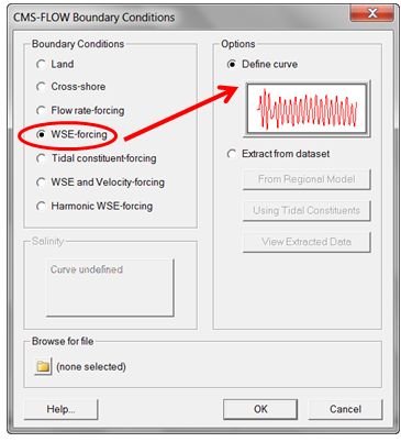
For many coastal applications, a single water level time-series curve is sufficient. Water level measurements are usually obtained from a nearby tidal gauge. A water level time series can be specified in the ''CMS-Flow Boundary Conditions'' window (see Figure below). | |||
[[File:fig_2-48.png]] | |||
Figure 2-48. Single water level time-series specification in SMS 11.1. | |||
Table 2-46. CMS-Flow cards related to the single water level time series boundary condition. | |||
{|class="wikitable" | |||
|- | |||
!Input | |||
!Format | |||
!Notes | |||
|- | |||
|WSE time series boundary | |||
|[card=HDRIVER_CELLSTRING] | |||
[name=Hfile, type=char, | |||
default=none] | |||
[name=Hpath, type=char, | |||
default=none] | |||
|Specifies the Boundary ID File and Path (if necessary). Outdated in CMS V4.1 and newer. Has been replaced by block structure format. | |||
|} | |||
Example 2-32. Single WSE time-series BC specification using a single card | |||
---- | |||
HDRIVER_CELLSTRING "Flow_Shark_mp.h5" "PROPERTIES/Model Params/Boundary_#1" | |||
---- | |||
=Note= | |||
:• Careful attention is needed when using a single water level time series. If the location of the measured water levels is far away from the model boundary, this may result in significant amplitude and phase errors. In some cases, if the errors or minor, it is possible to adjust the measured water levels by comparing measured and calculated water levels at other water level stations and adjusting the reference time and scaling the amplitude of the measured water level time series. However, this approach is very simplistic and caution should always. If the amplitude or phase errors are significant it not recommended to attempt any corrections and instead use a tidal database to force the model. | |||
=Tips= | |||
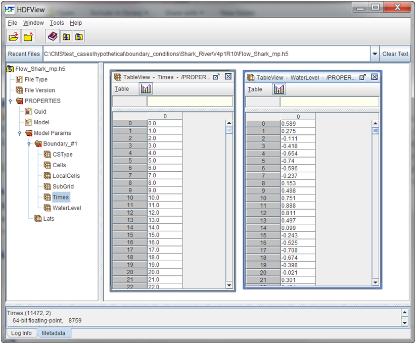
:• It is recommended to install and use HDFView to view the CMS XMDF files. HDFView can be used to open and even edit the boundary condition data without opening SMS. The figure below shows an example of a CMS-Flow Model Parameters File with a single water level time series curve specified. The data tree on the left-hand-side can be expanded to explore the datasets. In the figure below, the datasets for the water level times and values are shown. | |||
[[File:fig_2-49.png]] | |||
Figure 2-49. Single Water Level Time Series data structure within the CMS-Model Parameters File. | |||
=Step-by-Step Instructions: Assigning a Single Water Level Time Series= | |||
This is the option called Define Curve in SMS. In this BC, a single time series of water levels is specified and is applied at all of the cells along a boundary cell string. The time series curve may be specified by either im-porting an SMS *.xys file, copying tabular data into SMS, or manually en-tered the time series information in SMS. To assign this type of BC in SMS | |||
:1. If not already done, load a CMS-Flow grid in SMS. | |||
:2. If not already created by SMS, create the cellstring at the boundary (see section ''Creating and Deleting Cell Strings in SMS'' for details). | |||
:3. Select the cellstring (see section ''Selecting a Cellstring'' for details) and | |||
:4. Open the CMS-Flow Boundary Conditions Window (see section ''Assigning a Boundary Condition'' for details). See Figure 2-50. | |||
[[File:fig_2-50.png]] | |||
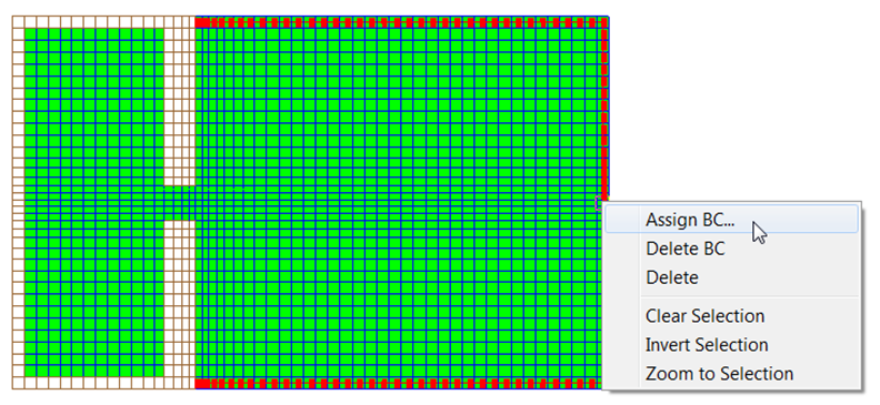
Figure 2 50. Selecting the cellstring along the ocean boundary, and clicking on Assign BC. | |||
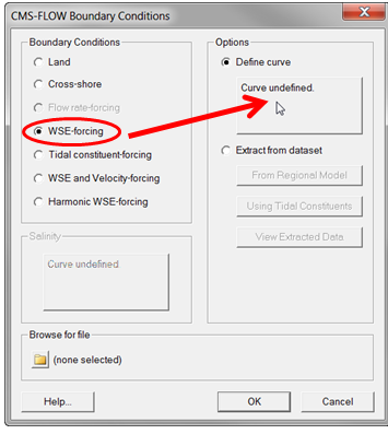
:5. Select the ''WSE-forcing'' boundary condition, and click curve unde-fined (see Figure 2-50) under ''Define Curve''. | |||
[[File:fig_2-51.png]] | |||
Figure 2-51. Defining the single water surface elevation curve. | |||
:6. The ''XY Series Editor'' will open. | |||
:7. Enter the time-series data in the left side of the window either by | |||
::a. Copy-pasting a time series from a spreadsheet, | |||
::b. Manually entering the times and WSE values, or | |||
::c. Importing an SMS xys file by clicking on the ''Import''… button in which the SMS interface will prompt the user to select the appropriate file. | |||
:8. The time series should appear in the plot on the right-side of the window (see figure below). | |||
[[File:fig_2-52a.png]] | |||
[[File:fig_2-52b.png]] | |||
Figure 2-52. Top: is the blank XY Series Editor; Bottom: after the data is pasted in. | |||
:9. If the user selects to, the boundary time series may be saved to a file by click ingon the ''Export''… button. | |||
:10. Save the ''SMS project File'' (*.sms) or ''CMS-Flow Simulation File'' (*.cmcards). | |||
=Notes= | |||
:• When importing an SMS xys file, it is important to note that the SMS reads the file and loads the data rather than linking to that file. If the file is changed, the boundary condition in SMS will NOT automatically update. | |||
:• The water level time series do not have to have regular spacing. | |||
:• The water level time series should cover the time extent of the simulation. If the time series does not the model will still run and use the nearest value from time series. | |||
=Tips= | |||
:• When specifying the time series forcing in SMS manually or by copying from an spreadsheet, it is recommended to save the time series forcing in SMS XY Series Files (*.xys). If a new grid is cre-ated, the file can be easily reloaded in SMS. In addition, these files serve as a record of the model forcing; serve as a backup in case the Model Parameters File becomes corrupt. | |||
:• For most coastal applications it a time series interval of about 5 to 30 minutes is sufficient. | |||
=Extracted Water Level Time Series Boundary= | |||
This BC type is named ''Extract from dataset'' in SMS 11.0 and 11.1 (see figure below). In this boundary condition type, an individual water level time-series is specified for each boundary cell. The SMS interface allows the user to extract these time series from a larger CMS or ADCIRC simulation or to synthesize them from interpolated tidal constituents from a tidal database. | |||
[[File:fig_2-53.png]] | |||
Figure 2-53. CMS-Flow Boundary Conditions window in SMS 11.1 with an assigned WSE-Forcing from an extracted dataset. | |||
The CMS-Flow card used to specify the extracted water level boundary condition is described in the table below. | The CMS-Flow card used to specify the extracted water level boundary condition is described in the table below. | ||
Table 2-47. CMS-Flow cards related to the extracted water level time series boundary condition. | |||
{|class="wikitable" | |||
|- | |||
!Input | |||
!Format | |||
!Notes | |||
|- | |||
|Extracted WSE time series boundary | |||
|[card=MDRIVER_CELLSTRING] | |||
[name=MHfile, type=char, | |||
default=none] | |||
[name=MHpath, type=char, | |||
default=none] | |||
|Specifies the Boundary ID File and Path (if necessary). | |||
|} | |||
Latest revision as of 18:26, 7 May 2015
Figure 2-47. CMS-Flow Boundary Conditions Window in SMS 11.1
Wall Boundary
The wall boundary condition is a closed boundary and is applied at any cell face between wet and dry cells. Any unassigned boundary cells at the edge of the model domain are assumed to be closed and are assigned a wall boundary. A zero normal flux to the boundary is applied at closed boundaries. Two boundary conditions are available for the tangential flow
- 1. Free-slip: No tangential shear stress (wall friction)
- 2. Partial-slip: Tangential shear stress (wall friction) calculated based on the log-law
Assuming a log-law for a rough wall, the partial-slip tangential shear stress is given by
| (2-10) |
where is the magnitude of the wall parallel current velocity and cwall is the wall friction coefficient equal to
| (2-11) |
Here y0 is the roughness length of the wall and is assumed to be equal to that of the bed (i.e. y0 = z0 ). ypis the distance from the wall to the cell center.
Notes
- • When SMS generates a new grid, cellstrings are automatically generated along all boundaries. The default boundary type is the wall boundary. It is recommended to delete all boundary cellstrings which are not open boundary conditions, since the wall boundary conditions are automatically assigned within the model. Deleting the cellstrings avoids confusion when assigning the boundary con-ditions.
- • Since the wall boundary is a closed boundary and all unassigned boundaries are treated as closed, the wall boundary cellstring in-formation does not need to written to the CMS-Flow Card File.
Flux Boundary
The flux boundary condition is typically applied to the upstream end of a river or stream and is specified as either a constant or time-series of total water volume flux. In a 2DH model, the total volume flux needs to be distributed across the boundary in order to estimate the depth-averaged velocities. This is done using a conveyance approach in which the current velocity is assumed to be related to the local flow depth h and Manning’s n as (i.e. ). Here r is an empirical conveyance coefficient equal to approximately 2/3 for uniform flow. The smaller the value the more uniform the current velocities are across the flux boundary. The water volume flux, qi , at each boundary cell i is calculated as
| (2-12) |
where
- i = subscript indicating a boundary cell
- = volume discharge at boundary cell i per unit width [m2/s]
- = unit vector for inflow direction = (sin )
- = inflow direction measured clockwise from North [deg]
- = boundary face unit vector (positive outward)
- Q = total volume flux across the boundary [m3/s]
- n = Manning’s coefficient [s/m1/3]
- r =empirical constant equal to approximately 2/3
- =cell width in the transverse direction to flow [m]
- fRamp = ramp function [-]
The total volume flux is positive into the computational domain. Since it is not always possible to orient all flux boundaries to be normal to the flux boundaries, the option is given to specify an inflow direction . The angle is specified in degrees clockwise from true North. If the angle is not specified, then the inflow angle is assumed to be normal to the boundary. The total volume flux is conserved independently of the inflow direction.
As mentioned above, the total water volume flux QB may be specified as a constant value or a single time-series curve. A description of the CMS-Flow cards used to specify the flux boundary condition information is provided in the table below.
Table 2-42. CMS-Flow cards related to the flux boundary condition.
| Input | Format | Notes |
|---|---|---|
| Flux boundary | [card=QDRIVER_CELLSTRING]
[name=Qfile, type=char, default=none] [name=Qpath, type=char, default=none] |
Specifies the Boundary ID File and Path (if necessary). Outdated in CMS V4.1 and newer. Has been replaced by block structure format. |
Example 1: Single line flux boundary specification
QDRIVER_CELLSTRING "Flow_mp.h5" "PROPERTIES/Model Params/Boundary"
Step-by-Step Flux Boundary Specification in SMS
The flow rate boundary condition specifies a time series of water fluxes in units of m3/s per cell. To assign a flux BC in SMS
- 1. If not already created by SMS, create the cellstring at the flux boundary (see section Creating and Deleting Cell Strings in SMS for details).
- 2. Select the cellstring (see section Selecting a Cellstring for details)
- 3. Open the CMS-Flow Boundary Conditions Window (see section Assigning a Boundary Condition for details).
- 4. Enter a time series of total flux values on and select OK button.
- 5. Save the SMS project File (*.sms) or CMS-Flow Simulation File (*.cmcards).
Total flow rate specified is divided between the total number of cells in the cellstring with each assigned a portion of the total flux as function of the local water depth and bottom friction.
Notes
- • The flux boundary type may ONLY be specified along cellstrings which are straight (i.e. the cellstring may not wrap around corners).
- • Cellstrings have to be at least three cells long.
- • Positive fluxes are directed inward and negative fluxes are directed outward. By default the inflow/outflow angles are assumed to be normal to the boundary. The angle may be changed using the ad-vanced block structure described in the following section.
- • If the flux data file name and path are not specified, then they are assumed to be the same as for cellstring.
Water Level Boundaries
The water level at a boundary can be specified as
- 1. Constant value
- 1. Single time-series curve
- 2. Cell-specific time-series curves (i.e. one time-series for each boundary cell)
- 3. Tidal constituents
- 4. Harmonic constituents
- 5. Extracted values from a parent grid simulation (nesting)
- 6. Tidal database
The general formula for the boundary water surface elevation is given by
| (2-13) |
where
- = boundary water surface elevation [m]
- = external boundary water surface elevation [m]
- = water surface elevation offset [m]
- = initial boundary water surface elevation [m]
- = correction to the boundary water surface elevation which is a function of the wind and wave forcing [m]
- = water surface elevation component derived from user speci-fied gradients [m]
- fRamp= ramp function [-]
The external water surface elevation may be spatially and temporally con-stant or variable. When a time series is specified, the values are interpolated using piecewise Lagrangian polynomials. By default, second order interpolation is used, but can be changed by the user. The water surface elevation offset is assumed spatially and temporally constant and may be used to correct the boundary water surface elevation for vertical datums, surge, and sea level rise. The correction is only applicable when is spatially constant as in the case of a single water surface elevation time-series. The component is intended to represent regional gradients in the water surface elevation, is assumed to be constant in time, and is only applicable when is spatially constant.
A small degree of relaxation is obtained by applying the water level forcing as a source term rather than assigning the water level at the boundaries. This technique is common practice in finite volume models and improves stability and convergence. When applying a water level boundary condition to the nearshore, local flow reversals and boundary problems may result if the wave-and wind-induced setup are not included. This problem is avoided by adjusting the local water level to account for the cross-shore wind and wave setup similar that described in Reed and Militello (2005).
Tidal Boundary
Tidal or astronomic water level predictions are based on the official United States National Oceanographic and Atmospheric Administration (NOAA) Tides and Currents website: http://tidesandcurrents.noaa.gov and using the National Ocean Service (NOS) (http://co-ops.nos.noaa.gov) prediction formula
| (2-14) |
where
- i = subscript indicating a tidal constituent
- Ai= mean amplitude [m]
- fi= node (nodal) factor [-]
- = frequency [deg/hr]
- t = elapsed time from midnight of the starting year [hrs]
- = equilibrium phase [deg]
- = phase lag or epoch [deg]
The nodal factor is a time-varying correction to the mean amplitude. The equilibrium phase has a uniform component and a relatively smaller periodic component. The zero-superscript of indicates that the constituent phase is at time zero. The table below provides a list of tidal constituents currently supported in CMS. More information on U.S. tidal constituent values can be obtained from NOAA and NOS.
Table 2-43. Tidal Constituents names (cname) and speeds (in degrees per solar hour) implemented in CMS.
| Constituent | Speed | Constituent | Speed | Constituent | Speed | Constituent | Speed |
|---|---|---|---|---|---|---|---|
| SA* | 0.041067 | SSA* | 0.082137 | MM* | 0.54438 | MSF* | 1.0159 |
| MF* | 1.098 | 2Q1* | 12.8543 | Q1* | 13.3987 | RHO1* | 13.4715 |
| O1* | 13.943 | M1* | 14.4967 | P1* | 14.9589 | S1* | 15.0 |
| K1* | 15.0411 | J1* | 15.5854 | OO1* | 16.1391 | 2N2* | 27.8954 |
| MU2* | 27.9682 | N2* | 28.4397 | NU2* | 28.5126 | M2 | 28.9841 |
| LDA2* | 29.4556 | L2* | 29.5285 | T2* | 29.9589 | S2 | 30 |
| R2* | 30.0411 | K2 | 30.0821 | 2SM2* | 31.0159 | 2MK3* | 42.9271 |
| M3* | 43.4762 | MK3* | 44.0252 | MN4* | 57.4238 | M4 | 57.9682 |
| MS4* | 58.9841 | S4* | 60.0 | M6 | 86.9523 | S6* | 90.0 |
| M8* | 115.9364 |
*Only available through advanced cards for CMS >v4.0
Table 2-44. CMS-Flow Cards related to the Tidal Boundary specification.
| Input | Format | Notes |
|---|---|---|
| Begins a Tidal
Constituents Boundary Block |
[begin=TIDAL_CONSTITUENTS_BEGIN,
name=TCblock] |
Begins the block structure for a flux boundary condition |
| Tidal constituent card time series file | [card=TIDAL_CONSTITUENT_(cname),
parent=TCblock] [name=WSEfile, type=char, default=none] [name=WSEpath, type=char, parent=WSEblock, default=none] |
Specifies the WSE Data File Name (including path if different from Card File) and Dataset Path (for XMDF files only). Optional. Assumed to be the same as the cellstring if not specified. The file must contain a time-series for each boundary cell. |
| Ends Tidal
Constituents Boundary Block |
[end=TIDAL_CONSTITUENTS_END,
name=TCblock] |
Ends the block structure for a flux boundary condition |
| Tidal boundary
cellstring |
[card=TIDAL_CELLSTRING]
[name=Hfile, type=char, default=none] [name=Hpath, type=char, default=none] |
Specifies the Boundary ID File and Path (if necessary). Outdated in CMS V4.1 and newer. Has been replaced by block structure format. |
In the example below, the amplitude and phase of tidal constituents are specified. The tidal constituents are assigned to the tidal boundary condi-tion specified by the TIDAL_CELLSTRING card.
Example 2-30. Tidal boundary condition specification.
TIDAL_CONSTITUENTS_BEGIN
  TIDAL_CONSTITUENT_M2   0.75 211.0  ![Amplitude (m)] [Phase (deg)]
  TIDAL_CONSTITUENT_S2   0.18 231.0  ![Amplitude (m)] [Phase (deg)]
  TIDAL_CONSTITUENT_K1   0.15 185.0  ![Amplitude (m)] [Phase (deg)]
  TIDAL_CONSTITUENT_O1   0.24 191.0  ![Amplitude (m)] [Phase (deg)]
TIDAL_CONSTITUENTS_END TIDAL_CELLSTRING "Flow_mp.h5" "PROPERTIES/Model Params/Boundary"
Notes
- • The order of the tidal constituents does not matter.
- • In the example above the tidal constituent cards are indented for better readability. He SMS interface version 11.1 and earlier do not indent these cards. The model is not sensitive to the amount of indentation.
- • It is only possible to assign one tidal boundary condition using this card format. In order to have more than one tidal boundary condi-tion, the advanced cards must be used described in Section “Advanced Boundary Specification”.
Harmonic Boundary
If a harmonic boundary condition is applied, then the node factors are set to 1.0 and the equilibrium arguments are set to zero. Similarly to the water level boundary condition, the local water level at the boundary is adjusted to account for the wind and wave setup in order to avoid local flow reversals or instabilities (Reed and Militello 2005).
| (2-15) |
where
- i = subscript indicating a tidal constituent
- Ai= mean amplitude [m]
- = frequency [deg/hr]
- t = elapsed time from midnight of the starting year [hrs]
- = phase [deg]
The nodal factor is a time-varying correction to the mean amplitude The equilibrium phase has a uniform component and a relatively smaller periodic component. The zero-superscript of indicates that the constituent phase is at time zero.
Table 2-45. CMS-Flow Cards related to the Harmonic Boundary specification.
| Input | Format | Notes |
|---|---|---|
| Begins a Harmonic
Boundary Block |
[begin=HARMONIC_BEGIN,
name=Harmblock] |
Begins the block structure for a flux boundary condition |
| Harmonic component amplitude, phase, and speed | [card=HARMONIC_COMPONENT_(HarmJ),
parent=Harmblock)] [arg=HarmAmp(HarmJ), type=real, parent=Harmblock, default=none] [arg=HarmPha(HarmJ), type=real, parent= Harmblock,default=none] |
Specifies the harmonic component amplitude (m), phase (deg), and speed (deg/hr). HarmJ is an integer indicating the harmonic component. |
| Ends a Harmonic
Boundary Block |[end=HARMONIC_END, name=TCblock] |
Ends the block structure for a flux boundary condition | |
| Harmonic boundary
cellstring |
[card=HARMONIC_CELLSTRING]
[arg=Hfile, type=char, default=none] [arg=Hpath, type=char, default=none] |
Specifies the Boundary ID File and Path (if necessary). Outdated in CMS V4.1 and newer. Has been replaced by block structure format. |
Example 2-31. Harmonic boundary condition specification (SMS 11.1).
HARMONIC_BEGIN
  HARMONIC_COMPONENT_1  1.0  0.0 28.9841 ![Amp(m)] [Phase(deg)] [Speed(º/hr)]
  HARMONIC_COMPONENT_2  0.5 20.0 30.000  ![Amp(m)] [Phase(deg)] [Speed(º/hr)]
HARMONIC_END HARMONIC_CELLSTRING "Flow_mp.h5" "PROPERTIES/Model Params/Boundary"
Notes
- • The phases used in the harmonic boundary conditions are specified with respect to the start of the simulation.
- • The speeds for the major tidal constituents can be found on the NOAA Tides and Currents Website: http:// http://tidesandcurrents.noaa.gov/.
Water Level Time Series Curve
For many coastal applications, a single water level time-series curve is sufficient. Water level measurements are usually obtained from a nearby tidal gauge. A water level time series can be specified in the CMS-Flow Boundary Conditions window (see Figure below).
Figure 2-48. Single water level time-series specification in SMS 11.1.
Table 2-46. CMS-Flow cards related to the single water level time series boundary condition.
| Input | Format | Notes |
|---|---|---|
| WSE time series boundary | [card=HDRIVER_CELLSTRING]
[name=Hfile, type=char, default=none] [name=Hpath, type=char, default=none] |
Specifies the Boundary ID File and Path (if necessary). Outdated in CMS V4.1 and newer. Has been replaced by block structure format. |
Example 2-32. Single WSE time-series BC specification using a single card
HDRIVER_CELLSTRING "Flow_Shark_mp.h5" "PROPERTIES/Model Params/Boundary_#1"
Note
- • Careful attention is needed when using a single water level time series. If the location of the measured water levels is far away from the model boundary, this may result in significant amplitude and phase errors. In some cases, if the errors or minor, it is possible to adjust the measured water levels by comparing measured and calculated water levels at other water level stations and adjusting the reference time and scaling the amplitude of the measured water level time series. However, this approach is very simplistic and caution should always. If the amplitude or phase errors are significant it not recommended to attempt any corrections and instead use a tidal database to force the model.
Tips
- • It is recommended to install and use HDFView to view the CMS XMDF files. HDFView can be used to open and even edit the boundary condition data without opening SMS. The figure below shows an example of a CMS-Flow Model Parameters File with a single water level time series curve specified. The data tree on the left-hand-side can be expanded to explore the datasets. In the figure below, the datasets for the water level times and values are shown.
Figure 2-49. Single Water Level Time Series data structure within the CMS-Model Parameters File.
Step-by-Step Instructions: Assigning a Single Water Level Time Series
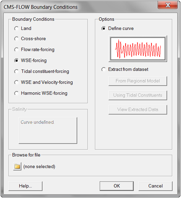
This is the option called Define Curve in SMS. In this BC, a single time series of water levels is specified and is applied at all of the cells along a boundary cell string. The time series curve may be specified by either im-porting an SMS *.xys file, copying tabular data into SMS, or manually en-tered the time series information in SMS. To assign this type of BC in SMS
- 1. If not already done, load a CMS-Flow grid in SMS.
- 2. If not already created by SMS, create the cellstring at the boundary (see section Creating and Deleting Cell Strings in SMS for details).
- 3. Select the cellstring (see section Selecting a Cellstring for details) and
- 4. Open the CMS-Flow Boundary Conditions Window (see section Assigning a Boundary Condition for details). See Figure 2-50.
Figure 2 50. Selecting the cellstring along the ocean boundary, and clicking on Assign BC.
- 5. Select the WSE-forcing boundary condition, and click curve unde-fined (see Figure 2-50) under Define Curve.
Figure 2-51. Defining the single water surface elevation curve.
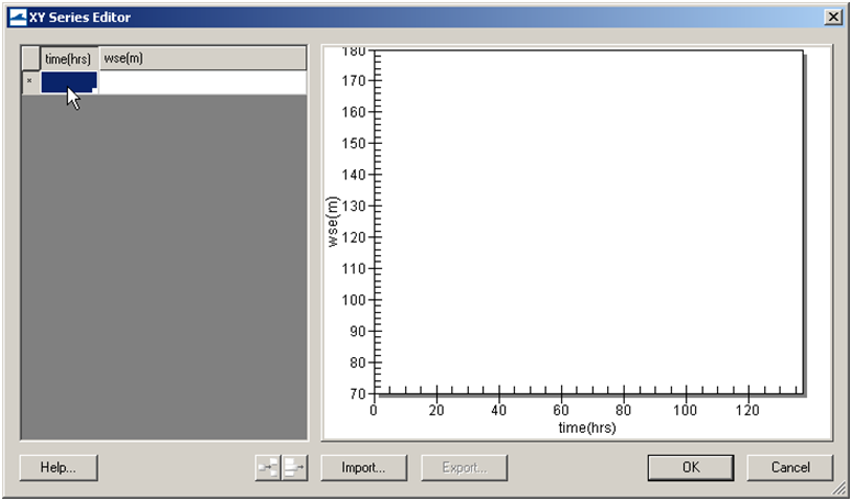
- 6. The XY Series Editor will open.
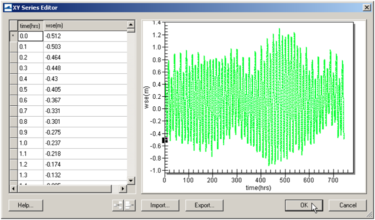
- 7. Enter the time-series data in the left side of the window either by
- a. Copy-pasting a time series from a spreadsheet,
- b. Manually entering the times and WSE values, or
- c. Importing an SMS xys file by clicking on the Import… button in which the SMS interface will prompt the user to select the appropriate file.
- 8. The time series should appear in the plot on the right-side of the window (see figure below).
Figure 2-52. Top: is the blank XY Series Editor; Bottom: after the data is pasted in.
- 9. If the user selects to, the boundary time series may be saved to a file by click ingon the Export… button.
- 10. Save the SMS project File (*.sms) or CMS-Flow Simulation File (*.cmcards).
Notes
- • When importing an SMS xys file, it is important to note that the SMS reads the file and loads the data rather than linking to that file. If the file is changed, the boundary condition in SMS will NOT automatically update.
- • The water level time series do not have to have regular spacing.
- • The water level time series should cover the time extent of the simulation. If the time series does not the model will still run and use the nearest value from time series.
Tips
- • When specifying the time series forcing in SMS manually or by copying from an spreadsheet, it is recommended to save the time series forcing in SMS XY Series Files (*.xys). If a new grid is cre-ated, the file can be easily reloaded in SMS. In addition, these files serve as a record of the model forcing; serve as a backup in case the Model Parameters File becomes corrupt.
- • For most coastal applications it a time series interval of about 5 to 30 minutes is sufficient.
Extracted Water Level Time Series Boundary
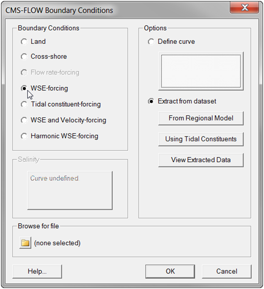
This BC type is named Extract from dataset in SMS 11.0 and 11.1 (see figure below). In this boundary condition type, an individual water level time-series is specified for each boundary cell. The SMS interface allows the user to extract these time series from a larger CMS or ADCIRC simulation or to synthesize them from interpolated tidal constituents from a tidal database.
Figure 2-53. CMS-Flow Boundary Conditions window in SMS 11.1 with an assigned WSE-Forcing from an extracted dataset.
The CMS-Flow card used to specify the extracted water level boundary condition is described in the table below.
Table 2-47. CMS-Flow cards related to the extracted water level time series boundary condition.
| Input | Format | Notes |
|---|---|---|
| Extracted WSE time series boundary | [card=MDRIVER_CELLSTRING]
[name=MHfile, type=char, default=none] [name=MHpath, type=char, default=none] |
Specifies the Boundary ID File and Path (if necessary). |


![{\displaystyle c_{wall}=\left[{\frac {\kappa }{ln(y_{p}/y_{0})-1}}\right]^{2}}](https://en.wikipedia.org/api/rest_v1/media/math/render/svg/519bd78855e265eb30944689417d919794bef3a6)


