User Guide 017: Difference between revisions
No edit summary |
No edit summary |
||
| (6 intermediate revisions by the same user not shown) | |||
| Line 51: | Line 51: | ||
Importing GIS-type files from D-ADCP current measurements output into SMS: | Importing GIS-type files from D-ADCP current measurements output into SMS: | ||
1. Open the provided file in the section folder SRI082009_DAV_1300.GIS, and select ''Use Import Wizard'' (An excel version of the text file is also provided in the folder). Select ''space/tab'' delimited if not already checked and click ''Next'', and select the X, Y, Z, Vector X and Vector Y col-umns (Figure 7 13). Be sure that the Header of the Vector X & Y columns is the same. Change the headers so they are the same (Vector), otherwise this incurs an error when importing in SMS. | :1. Open the provided file in the section folder SRI082009_DAV_1300.GIS, and select ''Use Import Wizard'' (An excel version of the text file is also provided in the folder). Select ''space/tab'' delimited if not already checked and click ''Next'', and select the X, Y, Z, Vector X and Vector Y col-umns (Figure 7 13). Be sure that the Header of the Vector X & Y columns is the same. Change the headers so they are the same (Vector), otherwise this incurs an error when importing in SMS. | ||
[[File:fig_7-13.png]] | [[File:fig_7-13.png]] | ||
| Line 75: | Line 75: | ||
[[File:fig_7-16.png]] | [[File:fig_7-16.png]] | ||
Figure 7 16. Color options turned on for scatter points. | Figure 7-16. Color options turned on for scatter points. | ||
To compare the measured current velocity data to calculated, the data must be in SMS in this format, where xyz data overlay the proper region and the units of the measurements are the same. Both datasets can be viewed and extracted within the SMS through the use of observation arcs. The arcs must be set along the transect line and have enough points to illicit one value per cell, but not too many where there will be duplicate calculated values. The imported measured datasets are much denser than the cell coverage. Below describes how to plot a transect, or observation arc, through the measured points that will display both measured point data and calculated data across a distance. | To compare the measured current velocity data to calculated, the data must be in SMS in this format, where xyz data overlay the proper region and the units of the measurements are the same. Both datasets can be viewed and extracted within the SMS through the use of observation arcs. The arcs must be set along the transect line and have enough points to illicit one value per cell, but not too many where there will be duplicate calculated values. The imported measured datasets are much denser than the cell coverage. Below describes how to plot a transect, or observation arc, through the measured points that will display both measured point data and calculated data across a distance. | ||
| Line 86: | Line 86: | ||
[[File:fig_7-17.png]] | [[File:fig_7-17.png]] | ||
Figure 7 17. Example of a feature arc with arrows in the ebb direction. Redistribute Vertices, Reverse Arc, and other options are available in the drop down menu. | Figure 7-17. Example of a feature arc with arrows in the ebb direction. Redistribute Vertices, Reverse Arc, and other options are available in the drop down menu. | ||
:3. To plot, select ''Plot Wizard'' from ''Display'', and select an ''Observation Profile''. In Step 2, select one of the arcs (uncheck others), and under ''Extra Profile'' select ''Model Intersections''. Figure 7-18 illustrates everything selected for plotting the measured and calculated data for the specific time of the transect measurement. | :3. To plot, select ''Plot Wizard'' from ''Display'', and select an ''Observation Profile''. In Step 2, select one of the arcs (uncheck others), and under ''Extra Profile'' select ''Model Intersections''. Figure 7-18 illustrates everything selected for plotting the measured and calculated data for the specific time of the transect measurement. | ||
| Line 108: | Line 108: | ||
Sediment transport roses are plots in which transport is integrated over directional bins and plotted over a map of the site in order to observe the amount and direction of sediment transport at a specific point. A general picture of the sediment transport pathways can be obtained by plotting several sediment transport roses in the areas of interest. Below is a step-by-step example for Shark River inlet on how to plot sediment transport roses: | Sediment transport roses are plots in which transport is integrated over directional bins and plotted over a map of the site in order to observe the amount and direction of sediment transport at a specific point. A general picture of the sediment transport pathways can be obtained by plotting several sediment transport roses in the areas of interest. Below is a step-by-step example for Shark River inlet on how to plot sediment transport roses: | ||
:1. Setup Observational Cells | |||
:2. Click on the [[File:335-1.png]] Select Cells tool. | |||
:3. Select a cell and left-click | |||
:4. Select Cell-attributes… (see Figure below). | |||
[[File:fig_7-20.png]] | |||
Figure 7-20. Opening the CMS-Flow Cell Attributes window. | |||
7. Run the model | The ''CMS-Flow Cell Attributes'' window will appear (see Figure below). | ||
8. Once the model has completed. The project folder will contain two files with the extension *_qtx.txt, and *_qty.txt. These files contain the total sediment transport rates in the x and y directions in units of kg/m/s. | |||
9. Plot the sediment transport roses in Matlab | :5. Check the box next to ''Transport output'', so that the model will output the sediment transport rates. | ||
10. Exporting a Georeferenced image in SMS | :6. Save the project | ||
[[File:fig_7-21.png]] | |||
Figure 7-21. CMS-Flow Cell Attributes window. | |||
Example observational cell cards: | |||
---- | |||
---- | |||
!Observation Cells | |||
TIME_SERIES_INCREMENT 900.0 | |||
FLOW_RATE_INCREMENT 900.0 | |||
Q_TRANS_RATE_INCREMENT 900.0 | |||
ELEV_OBS_CELLS_BEGIN | |||
22943 "North Beach" | |||
28784 "Bay" | |||
30926 "Bridge" | |||
ELEV_OBS_CELLS_END | |||
FLOW_OBS_CELLS_BEGIN | |||
22943 "North Beach" | |||
28784 "Bay" | |||
30926 "Bridge" | |||
FLOW_OBS_CELLS_END | |||
Q_TRANS_OBS_CELLS_BEGIN | |||
22943 "North Beach" | |||
28784 "Bay" | |||
30926 "Bridge" | |||
Q_TRANS_OBS_CELLS_END | |||
---- | |||
---- | |||
:7. Run the model | |||
:8. Once the model has completed. The project folder will contain two files with the extension *_qtx.txt, and *_qty.txt. These files contain the total sediment transport rates in the x and y directions in units of kg/m/s. | |||
:9. Plot the sediment transport roses in Matlab | |||
:10. Exporting a Georeferenced image in SMS | |||
If the grid is telescoping, it may be difficult to plot the grid in Matlab. There are ways of plotting a telescoping grid in Matlab, but for the purposes of visualization, the easiest approach is to export a georeferenced image from SMS and plot the image in Matlab. This is done by | If the grid is telescoping, it may be difficult to plot the grid in Matlab. There are ways of plotting a telescoping grid in Matlab, but for the purposes of visualization, the easiest approach is to export a georeferenced image from SMS and plot the image in Matlab. This is done by | ||
:1. Click on ''File | Save as''… (see Figure below) | |||
[[File:fig_7-22.png]] | |||
figure 7-23 | Figure 7-22. Opening the SMS Save As window. | ||
:2. Next to ''Save as type'', select JPEG Image File. | |||
:3. Navigate to the correct directory | |||
:4. Enter a file name | |||
:5. Click ''Save'' (see figure below). | |||
[[File:fig_7-23.png]] | |||
Figure 7-23. SMS Save As window. | |||
An image file will be saved along with a projection and world file. The projection file contains the horizontal projection information and the world file contains the coordinates of the image origin, the rotation angles (zero for SMS), and pixel size. The image file can easily be loaded and plotted in SMS. | An image file will be saved along with a projection and world file. The projection file contains the horizontal projection information and the world file contains the coordinates of the image origin, the rotation angles (zero for SMS), and pixel size. The image file can easily be loaded and plotted in SMS. | ||
Editing and running the Matlab script | |||
=Editing and running the Matlab script= | |||
The Matlab script below is just an example to show the basic steps in plotting the sediment transport roses in Matlab. For each application, the file names, directories, station ID’s, and settings will need to be modified. | The Matlab script below is just an example to show the basic steps in plotting the sediment transport roses in Matlab. For each application, the file names, directories, station ID’s, and settings will need to be modified. | ||
---- | |||
%Plots Sediment Transport Roses | |||
clear all | |||
%1. Obtain Observation Point coordinates | |||
id = [22943 28784 30926 33484 34145]; Station id's | |||
tel = read_cmstel('..\Hands-on\Flow_Shark.tel'); | |||
xsta = tel.x(id); ysta = tel.y(id); | |||
cosang = cos(tel.angle*pi/180); | |||
sinang = sin(tel.angle*pi/180); | |||
%2. Read transport vectors | |||
qtx = load('..\Hands-on\Flow_Shark_qtx.txt'); | |||
qty = load('..\Hands-on\Flow_Shark_qty.txt'); | |||
%3. Read and plot background image | |||
A = imread('..\Hands-on\Image_Shark2.jpg'); | |||
wld = load('..\Hands-on\Image_Shark2.wld'); | |||
xi = wld(5) + (0:size(A,2)-1)*wld(1); %SMS images are NOT rotated | |||
yi = wld(6) + (0:size(A,1)-1)*wld(4); | |||
imagesc(xi,yi,A) | |||
set(gca,'ydir','normal','Nextplot','add') | |||
%4. Plot roses, Rotate transports from local grid angle to world | |||
for k=1:size(qtx,2)-1 | |||
qte = qtx(:,k+1)*cosang - qty(:,k+1)*sinang; %East | |||
qtn = qtx(:,k+1)*sinang + qty(:,k+1)*cosang; %North | |||
[sumx,sumy] = sumdirbin(qte,qtn); | |||
x = ones(length(sumx),1)*xsta(k); | |||
y = ones(length(sumx),1)*ysta(k); | |||
h = vecplot(x,y,sumx,sumy,'marker','^',... | |||
'lengthscale',10,'linewidth',2,... | |||
'MarkerFaceColor','k','MarkerSize',3); | |||
end | |||
axis([1.9018 1.9257 1.4979 1.5132]*1e5) | |||
xlabel('X, State Plane, m'), ylabel('Y, State Plane, m') | |||
return | |||
The subroutine sumdirbin sums the transport rates over directional bins. Note that to integrate over time the values should also be multiplied by the output interval. However, because the vectors are only for plotting purposes, this step is not necessary here. The matlab script for summing the transports in directional bins is provided below | ---- | ||
The subroutine ''sumdirbin'' sums the transport rates over directional bins. Note that to integrate over time the values should also be multiplied by the output interval. However, because the vectors are only for plotting purposes, this step is not necessary here. The matlab script for summing the transports in directional bins is provided below | |||
---- | |||
function [binx,biny] = sumdirbin(u,v,binsize) | |||
% [binx,biny] = sumdirbin(u,v,varargin) | |||
% Sums the vector u,v in directional bins | |||
% written by Alex Sanchez, USACE | |||
if nargin<3 | |||
binsize = 22.5; %deg, default bin size | |||
end | |||
u = u(:); v = v(:); | |||
mag = sqrt(u.^2+v.^2); | |||
binlim = (-binsize/2:binsize:360-binsize/2)'; %limits | |||
bincen = (0:binsize:360-binsize)'; %centers | |||
ndir = length(binlim); | |||
angle = atan2(v,u)*180/pi; | |||
angle = mod(angle,360)+0.00001; | |||
angle(angle==0) = 0.00001; | |||
binmag = zeros(ndir-1,1); | |||
for k=1:ndir-1 | |||
ind = (angle>binlim(k) & angle<=binlim(k+1)); | |||
binmag(k) = sum(mag(ind)); | |||
end | |||
binx = binmag.*cos(bincen.*pi/180); | |||
biny = binmag.*sin(bincen.*pi/180); | |||
return | |||
---- | |||
The resulting Matlab plot is shown in the figure below. | The resulting Matlab plot is shown in the figure below. | ||
[[File:fig_7-24.png]] | |||
Figure 7-24. Total-load Sediment transport rates for Shark River Inlet. | |||
=Calculating Sediment Fluxes across Observational Arcs= | |||
In the CMS, sediment transport can be calculated across lines or polygons defined by feature arcs and polygons in a post-processing procedure. The integration across an arc may be written as | In the CMS, sediment transport can be calculated across lines or polygons defined by feature arcs and polygons in a post-processing procedure. The integration across an arc may be written as | ||
1. Set the Sediment Transport Simulation Statistics (see section Simulation Statistics for more details). | {{Equation|<math>\bar{Q}_t = \oint_L \frac{1}{T} \int_t (\overrightarrow{q}_t \cdot | ||
2. Run the CMS with sediment transport. | \overrightarrow{n}) dt \ dL</math>|7-1}} | ||
3. Load the XMDF Global Solution File into SMS (drag-and-drop is the easiest way). | |||
The data tree will have several sediment transport statistics including the Gross and Net Total-load sediment transport rates in units kg/m/s. Figure 7 25 shows an example of the data tree with the sediment simulation statistics for Shark River inlet. | where <math>\overrightarrow{q}_t </math> is the total-load sediment transport rate vector, ''t'' is time, ''L'' is the arc length, and <math>\overrightarrow{n} </math> is the unit vector normal to the arc line. Note that the order of the above integrals is irrelevant; however it is more efficient and accurate to perform the temporal integration first. CMS has the option to output sediment transport statistics which includes the net total-load sediment transport rate which is basically the temporal integration shown in the equation above. For further details on the sediment statistics see section <span style="color:#0000FF">Simulation Statistics</span>. To use the sediment statistics in calculating fluxes across observational arcs: | ||
:1. Set the Sediment Transport Simulation Statistics (see section <span style="color:#0000FF">Simulation Statistics <span> for more details). | |||
:2. Run the CMS with sediment transport. | |||
:3. Load the XMDF Global Solution File into SMS (drag-and-drop is the easiest way). | |||
The data tree will have several sediment transport statistics including the Gross and Net Total-load sediment transport rates in units kg/m/s. Figure 7-25 shows an example of the data tree with the sediment simulation statistics for Shark River inlet. | |||
[[File:fig_7-25.png]] | |||
Figure 7-25. Data tree showing the sediment and hydrodynamic simulation statistics. | |||
The total-load sediment transport rate is output into the Sed_Transp vec-tor and Sed_Transp_Net scalar datasets. Figure XX shows an example of the Net Total-load Sediment Transport vectors and magnitude after a short 24-hr simulation. | The total-load sediment transport rate is output into the Sed_Transp vec-tor and Sed_Transp_Net scalar datasets. Figure XX shows an example of the Net Total-load Sediment Transport vectors and magnitude after a short 24-hr simulation. | ||
[[File:fig_7-26.png]] | |||
Figure 7-26. Example of the Net Total-load Sediment Transport Rate vectors and magnitudes for Shark River inlet after a short 24-hr simulation. | |||
The datasets are output at start and end of the statistics period. The statistics at the initial time are always zero and are only necessary for SMS to be able to perform the line integral which is part of the Time Series plot (described further below). | The datasets are output at start and end of the statistics period. The statistics at the initial time are always zero and are only necessary for SMS to be able to perform the line integral which is part of the Time Series plot (described further below). | ||
:1. Either: | |||
::a. Create a new map coverage of Observation type or | |||
::b. Set the current map coverage to Observation type. | |||
[[File:fig_7-27.png]] | |||
Figure 7-27. Creating a new Map Coverage of type Obesrvation. | |||
[[File:fig_7-28.png]] | |||
Figure 7-28. Setting the current Map Coverage to an Observational type | |||
:2. Create an observational arc by selecting the Create Feature Arc Tool [[File:343-1.png]] , and click on the points that define the Observational arc (see Figure below). The example shown below is intended for longshore sediment transport. When calculating longshore sediment transport, the offshore end of the transects should extend beyond the breaker and closure depth. It is best that the ends of the observational arc do not touch inactive (land) cells as this may cause interpolation problems in SMS. | |||
[[File:fig_7-29.png]] | |||
Figure 7-29. Example of a Feature Arc for calculating sediment transport. | |||
3. If necessary, use the Select Feature Point | 3. If necessary, use the Select Feature Point [[File:344-1.png]] tool to adjust the end points of the arc (the arc can be deleted by selecting with the Select Feature Arc [[File:344-2.png]] tool and pressing the delete key). | ||
4. The positive direction of the sediment transport is defined by the Feature Arcs direction. To view the arc direction, click on the Select Feature Arc tool | 4. The positive direction of the sediment transport is defined by the Feature Arcs direction. To view the arc direction, click on the Select Feature Arc tool [[File:344-3.png]] and right-click on the Feature Arc once. The arrows displayed at the beginning and end of the transect indicate the direction of the arc which defines the positive for all fluxes or vectors calculated across it. | ||
Latest revision as of 20:22, 8 May 2015
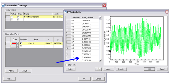
Figure 7-8. Input of time series water surface elevation data into an observation point.
Water level data plotting from Feature Points
Time plots can be compared within SMS through their software plotting package. To create a plot:
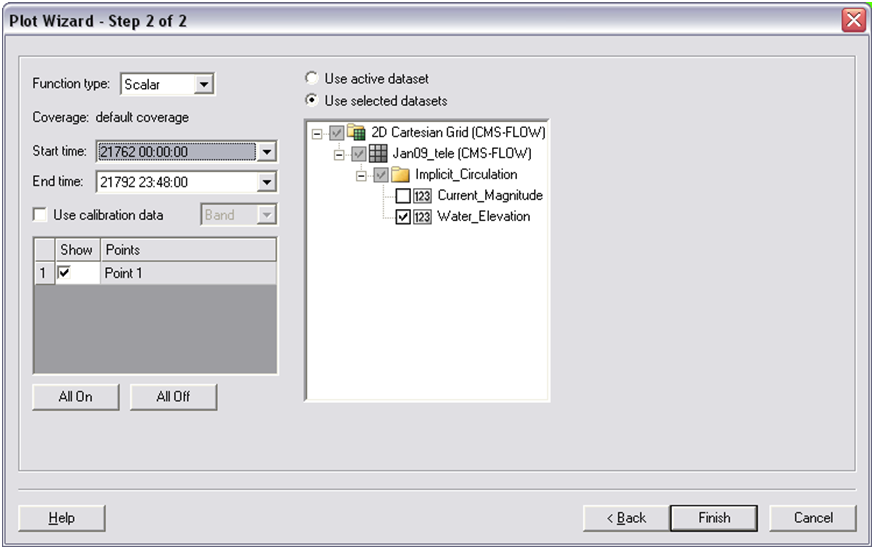
- 1. Select Display|Plot Wizard|Time Series and select Next. The Function is Scalar, and the Water Elevation scalar dataset should be selected with the full time period (Figure 4-59).
Figure 7-9. Plot Wizard for time series data (top); Time Series plot of Water Elevation (bottom).
- 2. The plots can be updated by right-clicking the graph window and selecting Plot Data. Also, the time frame can be modified.
- 3. Changing the location of the Feature Point by dragging the point will also automatically update any graph open within SMS. Note that moving Feature Points that are extracting large datasets may take a considerable amount of time to reload.
Extensive statistical analysis of time series water levels is not available in SMS. However, it is convenient to extract this information from SMS which can be used in other software or Microsoft Excel.
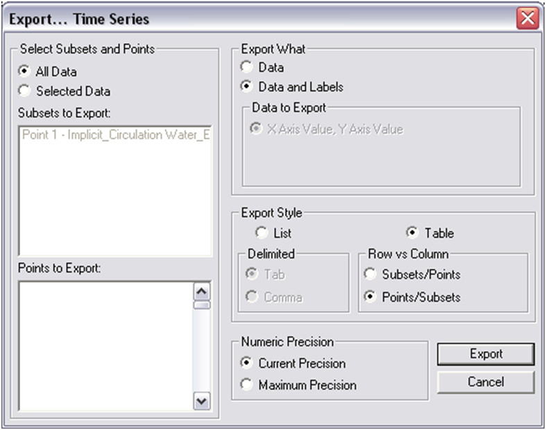
- 4. To extract the raw data for use in other software right-click on the graph window and select Export. In the Exporting Time Series window, select Export|Text/Data, Export Destination|File (and specify a location), and select Export. Change the Export Style to Table and Row vs. Column to Points/Subsets (Figure 4-60). Export.
Figure 7-10. Export Wizard for plotted data.
- 5. To view the raw data (and another way to extract) right-click on the graph window and select View Values. The data are presented in a table that can be highlighted and copied to another program.
Other options for the display plot can be found on the XMS Wiki (http://www.xmswiki.com/xms/SMS:2D_Plots).
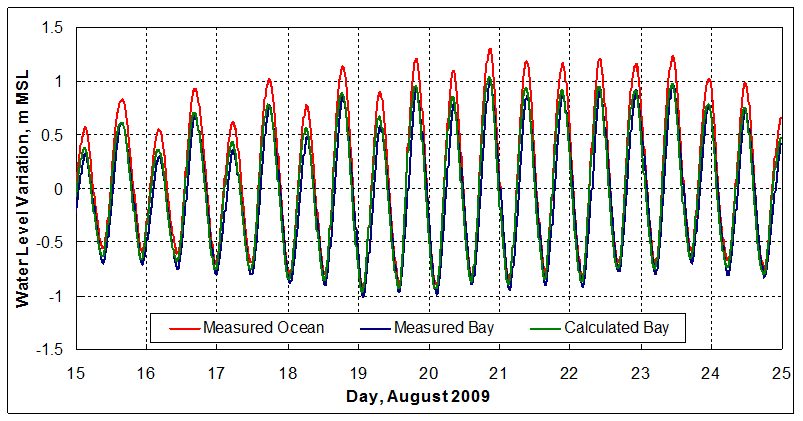
CMS-calculated water level variation is compared with water levels from the Belmar gauge (location shown in Figure 4-57) and given in Figure 7 11. Because the Sandy Hook gauge is located 30 km north of Shark River, the calculations have a slight phase advance in comparison to the measurements because the tidal wave propagates from north to south on this coast. The ocean gauge typically leads the bay gauge by 20-30 min.
Figure 7-11. Observed time series of water level at Sandy Hook and Belmar (“Bay”) and calculated water level at Belmar.
If time series data for the model were not set to the same interval as the measured data, there are filtering options within the data calculator. Reducing output (water level) from the solution:
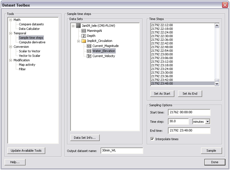
- 3. To create a 30 minute dataset of water levels from the origi-nal 6 minute output, go to Data, Data Calculator, and under the Tools section, select Temporal, Sample Time Steps (Figure 4-62).
Figure 7-12. Sampling time steps of the Water_Elevation scalar dataset in the Dataset Toolbox.
- 4. Select the water level dataset under the solution datatree, and create an Output dataset name at the bottom.
- 5. Set the Start time to the beginning of the series and the end time to the end by selecting the time under Time Steps and selecting the associated button below. Change the time step to 30 minutes (or 0.5 hours), select Sample.
Depth-average down-looking ADCP current data were measured at three transects, or 2-D profiles along transects, in Shark River Inlet during the calibration time period in August, 2009. This data was processed with off-the-shelf software, where velocity was binned into depth measurements throughout the water column, and converted into a .GIS file. To display preprocessed measured velocities, they must be converted into an XYZ format with additional data (velocity and direction, or Vx and Vy) in additional columns. SMS will recognize both the XYZ data, and assign extra scalar or vector datasets to the imported files.
Importing GIS-type files from D-ADCP current measurements output into SMS:
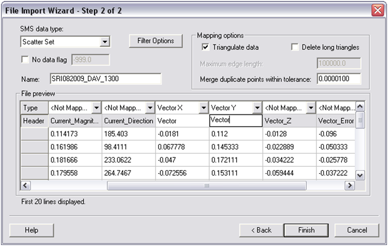
- 1. Open the provided file in the section folder SRI082009_DAV_1300.GIS, and select Use Import Wizard (An excel version of the text file is also provided in the folder). Select space/tab delimited if not already checked and click Next, and select the X, Y, Z, Vector X and Vector Y col-umns (Figure 7 13). Be sure that the Header of the Vector X & Y columns is the same. Change the headers so they are the same (Vector), otherwise this incurs an error when importing in SMS.
Figure 7-13. Sampling time steps of the Water_Elevation scalar dataset in the Dataset Toolbox.
All of the files were imported into SMS similarly as the time series data in the above section and are provided for you. All the data imported included X, Y, Z, Vx, Vy, Mag, and Dir for all three transects at a particular measurement time period. The files (under Hydro\Water Level Calibra-tion\Measured D-ave velocity GIS\SMS) have been converted into scatter datasets for quick import in SMS for viewing.
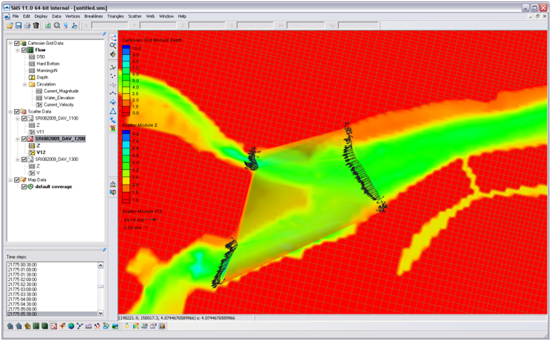
- 2. Import (drag and drop) one or two of the .h5 files (e.g. SHARK820_HOURLY - SRI082009_DAV_1100.h5). In Display Options, under Scatter, select velocity vectors and adjust the vector settings tab (Figure 7-14).
- 3. For a general estimate of comparison of the magnitude, convert one of the measurement files’ vectors to magnitude and direction (right click, vector to scalars). This can be compared to the calculated magnitude for a rough estimate.
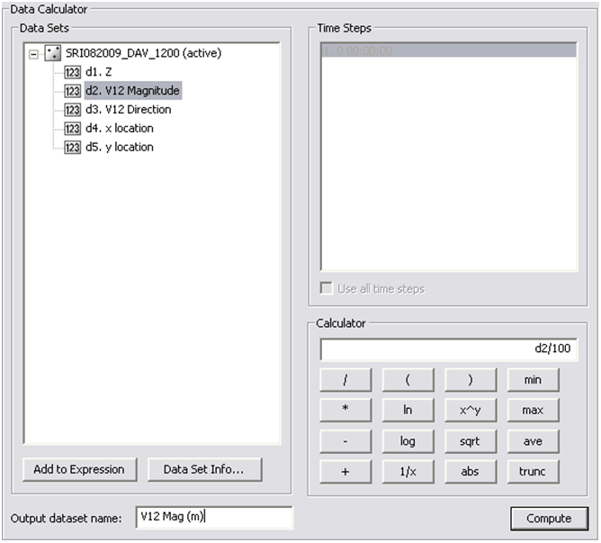
- 4. The scalar value of the measured data is in centimeters. Create a new dataset in meters using the data calculator (Figure 7-15).
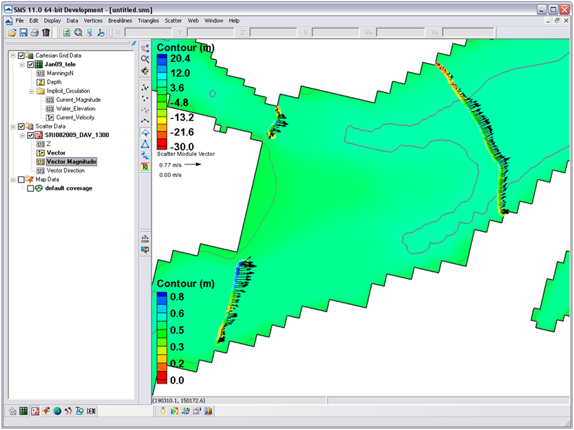
Figure 7-14. Example of the vector display along the measured transects. Note the vectors are scaled to the magnitude, and these scales can be manipulated in the Scatterset Vector tab.
Figure 7-15. Data calculator used to convert the vector magnitude from centimeters to meters for comparison to the calculated velocity magnitude.
- 6. To display the scatter points with colors representing the flow, go to the Scatter Tab under the Display Options, and select the Use Color Contour Scheme under Points. Make the points a size 10 and they will be visible and the color differences noticeable as in the figure below.
Figure 7-16. Color options turned on for scatter points.
To compare the measured current velocity data to calculated, the data must be in SMS in this format, where xyz data overlay the proper region and the units of the measurements are the same. Both datasets can be viewed and extracted within the SMS through the use of observation arcs. The arcs must be set along the transect line and have enough points to illicit one value per cell, but not too many where there will be duplicate calculated values. The imported measured datasets are much denser than the cell coverage. Below describes how to plot a transect, or observation arc, through the measured points that will display both measured point data and calculated data across a distance.
Displaying measured and calculated currents in SMS.
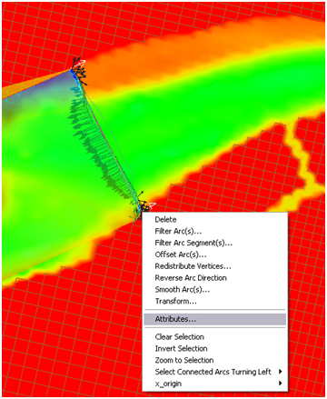
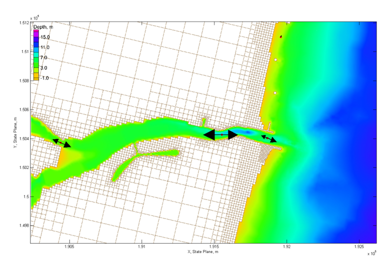
- 1. Following the above section, the current velocity file is displayed similar to Figure 7-17. Draw three observation arcs over each of the three transects. Directional arrows will display, and the direction of the arc should reflect ebbing or flooding. If the arrows face the flooding direction, flood currents will be positive, and ebb currents will be negative.
- 2. Redistribute the vertices on the arcs (they should not have any yet) to a value similar to the number of cells across each tran-sect. E.g. Transect 1 (main channel) should have 25-30 vertices.
Figure 7-17. Example of a feature arc with arrows in the ebb direction. Redistribute Vertices, Reverse Arc, and other options are available in the drop down menu.
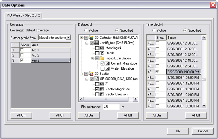
- 3. To plot, select Plot Wizard from Display, and select an Observation Profile. In Step 2, select one of the arcs (uncheck others), and under Extra Profile select Model Intersections. Figure 7-18 illustrates everything selected for plotting the measured and calculated data for the specific time of the transect measurement.
Figure 7-18. Plot Wizard data options for displaying measured and calculated data from an observation arc.
- 4. Specify the datasets to be plotted, the Current_Magnitude under the grid and the Vector Magnitude under the scatterset data. Select the date and time the transect was measured, which was 20 August 2009 at 1PM GMT.
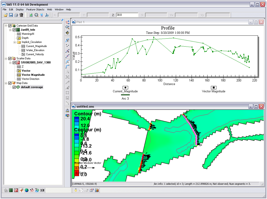
- 5. The resultant plot is shown in Figure 7-19, where the closest points from the measured data were plotted as distance across the arc, and model grid cell centers are where numbers are ex-tracted for the calculated data. Data can be extracted from the plot similarly to the ways defined in the water level extraction section at the beginning of this section.
Figure 7-19. Plotted measured and calculated data from the larger observation arc to the East. Note that the positive direction reflects the observation arcs direction.
Sediment Transport
Sediment transport rates can be used to calculate sediment statistics, sediment pathways, fluxes across arcs, and balances over polygonal areas. Several sediment transport statistics can be calculated during the simula-tion and output at any time. These statistics include the net and gross total sediment transport rates. For additional details see the Simulation Statistics section.
Calculating Sediment Transport Roses at Observation (Save) Points
Sediment transport roses are plots in which transport is integrated over directional bins and plotted over a map of the site in order to observe the amount and direction of sediment transport at a specific point. A general picture of the sediment transport pathways can be obtained by plotting several sediment transport roses in the areas of interest. Below is a step-by-step example for Shark River inlet on how to plot sediment transport roses:
- 1. Setup Observational Cells
- 2. Click on the
 Select Cells tool.
 - 3. Select a cell and left-click
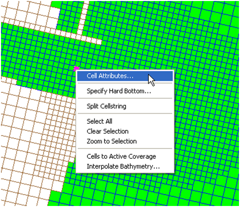
- 4. Select Cell-attributes… (see Figure below).
Figure 7-20. Opening the CMS-Flow Cell Attributes window.
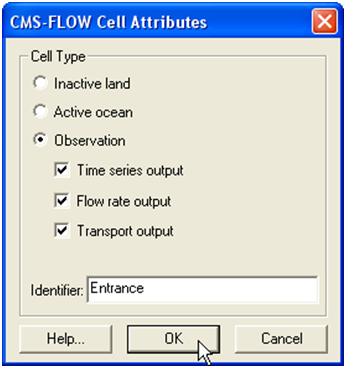
The CMS-Flow Cell Attributes window will appear (see Figure below).
- 5. Check the box next to Transport output, so that the model will output the sediment transport rates.
- 6. Save the project
Figure 7-21. CMS-Flow Cell Attributes window.
Example observational cell cards:
!Observation Cells TIME_SERIES_INCREMENT 900.0 FLOW_RATE_INCREMENT 900.0 Q_TRANS_RATE_INCREMENT 900.0 ELEV_OBS_CELLS_BEGIN
    22943 "North Beach"
    28784 "Bay"
    30926 "Bridge"
ELEV_OBS_CELLS_END FLOW_OBS_CELLS_BEGIN
    22943 "North Beach"
    28784 "Bay"
    30926 "Bridge"
FLOW_OBS_CELLS_END Q_TRANS_OBS_CELLS_BEGIN
    22943 "North Beach"
    28784 "Bay"
    30926 "Bridge"
Q_TRANS_OBS_CELLS_END
- 7. Run the model
- 8. Once the model has completed. The project folder will contain two files with the extension *_qtx.txt, and *_qty.txt. These files contain the total sediment transport rates in the x and y directions in units of kg/m/s.
- 9. Plot the sediment transport roses in Matlab
- 10. Exporting a Georeferenced image in SMS
If the grid is telescoping, it may be difficult to plot the grid in Matlab. There are ways of plotting a telescoping grid in Matlab, but for the purposes of visualization, the easiest approach is to export a georeferenced image from SMS and plot the image in Matlab. This is done by
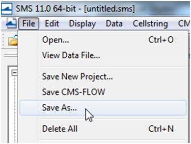
- 1. Click on File | Save as… (see Figure below)
Figure 7-22. Opening the SMS Save As window.
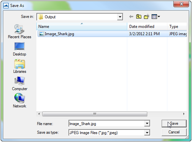
- 2. Next to Save as type, select JPEG Image File.
- 3. Navigate to the correct directory
- 4. Enter a file name
- 5. Click Save (see figure below).
Figure 7-23. SMS Save As window.
An image file will be saved along with a projection and world file. The projection file contains the horizontal projection information and the world file contains the coordinates of the image origin, the rotation angles (zero for SMS), and pixel size. The image file can easily be loaded and plotted in SMS.
Editing and running the Matlab script
The Matlab script below is just an example to show the basic steps in plotting the sediment transport roses in Matlab. For each application, the file names, directories, station ID’s, and settings will need to be modified.
%Plots Sediment Transport Roses clear all %1. Obtain Observation Point coordinates id = [22943 28784 30926 33484 34145]; Station id's tel = read_cmstel('..\Hands-on\Flow_Shark.tel'); xsta = tel.x(id); ysta = tel.y(id); cosang = cos(tel.angle*pi/180); sinang = sin(tel.angle*pi/180); %2. Read transport vectors qtx = load('..\Hands-on\Flow_Shark_qtx.txt'); qty = load('..\Hands-on\Flow_Shark_qty.txt'); %3. Read and plot background image A = imread('..\Hands-on\Image_Shark2.jpg'); wld = load('..\Hands-on\Image_Shark2.wld'); xi = wld(5) + (0:size(A,2)-1)*wld(1); %SMS images are NOT rotated yi = wld(6) + (0:size(A,1)-1)*wld(4); imagesc(xi,yi,A) set(gca,'ydir','normal','Nextplot','add') %4. Plot roses, Rotate transports from local grid angle to world for k=1:size(qtx,2)-1
   qte = qtx(:,k+1)*cosang - qty(:,k+1)*sinang; %East
   qtn = qtx(:,k+1)*sinang + qty(:,k+1)*cosang; %North
   [sumx,sumy] = sumdirbin(qte,qtn);
   x = ones(length(sumx),1)*xsta(k);
   y = ones(length(sumx),1)*ysta(k);
   h = vecplot(x,y,sumx,sumy,'marker','^',...
       'lengthscale',10,'linewidth',2,...
       'MarkerFaceColor','k','MarkerSize',3);
end axis([1.9018 1.9257 1.4979 1.5132]*1e5) xlabel('X, State Plane, m'), ylabel('Y, State Plane, m') return
The subroutine sumdirbin sums the transport rates over directional bins. Note that to integrate over time the values should also be multiplied by the output interval. However, because the vectors are only for plotting purposes, this step is not necessary here. The matlab script for summing the transports in directional bins is provided below
function [binx,biny] = sumdirbin(u,v,binsize) % [binx,biny] = sumdirbin(u,v,varargin) % Sums the vector u,v in directional bins % written by Alex Sanchez, USACE if nargin<3
binsize = 22.5; %deg, default bin size
end u = u(:); v = v(:); mag = sqrt(u.^2+v.^2); binlim = (-binsize/2:binsize:360-binsize/2)'; %limits bincen = (0:binsize:360-binsize)'; %centers ndir = length(binlim); angle = atan2(v,u)*180/pi; angle = mod(angle,360)+0.00001; angle(angle==0) = 0.00001; binmag = zeros(ndir-1,1); for k=1:ndir-1
   ind = (angle>binlim(k) & angle<=binlim(k+1));
   binmag(k) = sum(mag(ind));
end binx = binmag.*cos(bincen.*pi/180); biny = binmag.*sin(bincen.*pi/180); return
The resulting Matlab plot is shown in the figure below.
Figure 7-24. Total-load Sediment transport rates for Shark River Inlet.
Calculating Sediment Fluxes across Observational Arcs
In the CMS, sediment transport can be calculated across lines or polygons defined by feature arcs and polygons in a post-processing procedure. The integration across an arc may be written as
| (7-1) |
where is the total-load sediment transport rate vector, t is time, L is the arc length, and is the unit vector normal to the arc line. Note that the order of the above integrals is irrelevant; however it is more efficient and accurate to perform the temporal integration first. CMS has the option to output sediment transport statistics which includes the net total-load sediment transport rate which is basically the temporal integration shown in the equation above. For further details on the sediment statistics see section Simulation Statistics. To use the sediment statistics in calculating fluxes across observational arcs:
- 1. Set the Sediment Transport Simulation Statistics (see section Simulation Statistics for more details).
- 2. Run the CMS with sediment transport.
- 3. Load the XMDF Global Solution File into SMS (drag-and-drop is the easiest way).
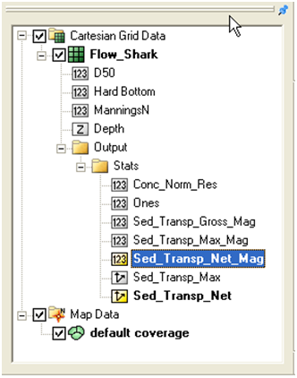
The data tree will have several sediment transport statistics including the Gross and Net Total-load sediment transport rates in units kg/m/s. Figure 7-25 shows an example of the data tree with the sediment simulation statistics for Shark River inlet.
Figure 7-25. Data tree showing the sediment and hydrodynamic simulation statistics.
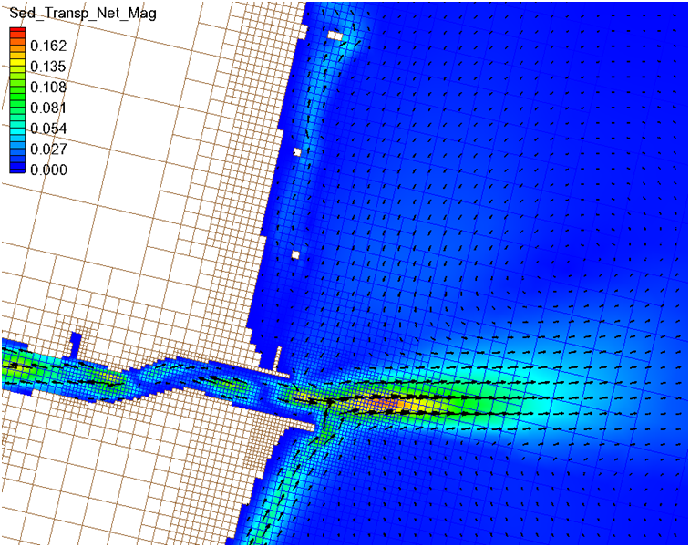
The total-load sediment transport rate is output into the Sed_Transp vec-tor and Sed_Transp_Net scalar datasets. Figure XX shows an example of the Net Total-load Sediment Transport vectors and magnitude after a short 24-hr simulation.
Figure 7-26. Example of the Net Total-load Sediment Transport Rate vectors and magnitudes for Shark River inlet after a short 24-hr simulation.
The datasets are output at start and end of the statistics period. The statistics at the initial time are always zero and are only necessary for SMS to be able to perform the line integral which is part of the Time Series plot (described further below).
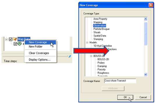
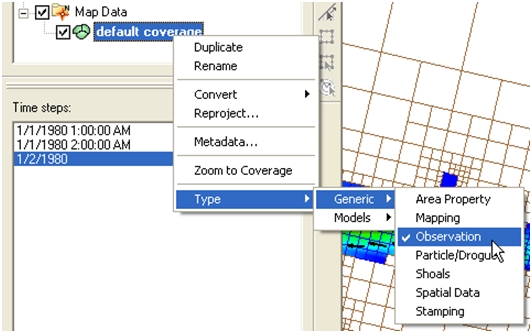
- 1. Either:
- a. Create a new map coverage of Observation type or
- b. Set the current map coverage to Observation type.
Figure 7-27. Creating a new Map Coverage of type Obesrvation.
Figure 7-28. Setting the current Map Coverage to an Observational type
- 2. Create an observational arc by selecting the Create Feature Arc Tool
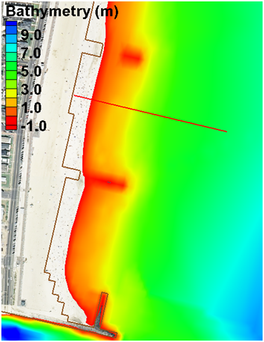
 , and click on the points that define the Observational arc (see Figure below). The example shown below is intended for longshore sediment transport. When calculating longshore sediment transport, the offshore end of the transects should extend beyond the breaker and closure depth. It is best that the ends of the observational arc do not touch inactive (land) cells as this may cause interpolation problems in SMS.
Figure 7-29. Example of a Feature Arc for calculating sediment transport.
3. If necessary, use the Select Feature Point ![]() tool to adjust the end points of the arc (the arc can be deleted by selecting with the Select Feature Arc
tool to adjust the end points of the arc (the arc can be deleted by selecting with the Select Feature Arc ![]() tool and pressing the delete key).
4. The positive direction of the sediment transport is defined by the Feature Arcs direction. To view the arc direction, click on the Select Feature Arc tool
tool and pressing the delete key).
4. The positive direction of the sediment transport is defined by the Feature Arcs direction. To view the arc direction, click on the Select Feature Arc tool ![]() and right-click on the Feature Arc once. The arrows displayed at the beginning and end of the transect indicate the direction of the arc which defines the positive for all fluxes or vectors calculated across it.
and right-click on the Feature Arc once. The arrows displayed at the beginning and end of the transect indicate the direction of the arc which defines the positive for all fluxes or vectors calculated across it.
