Shark River Inlet: Difference between revisions
| (17 intermediate revisions by 3 users not shown) | |||
| Line 1: | Line 1: | ||
<big> | <big> | ||
[[Image:Hands-on_SharkRiver_07.png|thumb|right|450px|Shark River Inlet]] | |||
[[Image:Hands-on_SharkRiver_07.png|thumb|right| | |||
==Introduction== | ==Introduction== | ||
| Line 21: | Line 14: | ||
4. Compare calculated channel morphology change to measured channel morphology | 4. Compare calculated channel morphology change to measured channel morphology | ||
The files and folders mentioned in this tutorial can be downloaded | |||
==Importing Bathymetric Datasets and Aerial Photographs== | ==Importing Bathymetric Datasets and Aerial Photographs== | ||
| Line 324: | Line 320: | ||
1. Download the NDBC standard monthly directional wave spectral file from | 1. Download the NDBC standard monthly directional wave spectral file from | ||
(e.g., 44025_200912) (Figures 28 to 31), this is provided under Hands On Materials - Shark River Inlet/Waves. | |||
[[Image:Shark_Fig29.PNG|thumb|right|400px|Figure 29. NODC buoy data access worldmap.]] | [[Image:Shark_Fig29.PNG|thumb|right|400px|Figure 29. NODC buoy data access worldmap.]] | ||
| Line 388: | Line 384: | ||
Importing CDIP buoy data is similar to the method of importing NDBC buoy data. | Importing CDIP buoy data is similar to the method of importing NDBC buoy data. | ||
1. Download the CDIP wave file | 1. Download the CDIP wave file ?nav=historic&sub=data (e.g., sp154-200912) (Figures 35 to 37), also provided under Hands On Materials - Shark River | ||
Inlet/Waves, | Inlet/Waves, | ||
| Line 688: | Line 684: | ||
<br style="clear:both" /> | <br style="clear:both" /> | ||
==== Loading Solution and Creating Obervation Arcs ==== | |||
[[Image:Shark_Fig62.PNG|thumb|right|400px|Figure 62. Shark River Inlet CMS-Flow grid with solution file loaded.]] | [[Image:Shark_Fig62.PNG|thumb|right|400px|Figure 62. Shark River Inlet CMS-Flow grid with solution file loaded.]] | ||
1. Load the ''Shark River Inlet-Workshop__Alt 1.cmcards'' into SMS by dragging it into the SMS or by clicking File <nowiki>|</nowiki> Open <nowiki>|</nowiki> ''Shark River Inlet-Workshop__Alt1.cmcards.'' The solution file should load in automatically. | 1. Load the ''Shark River Inlet-Workshop__Alt 1.cmcards'' into SMS by dragging it into the SMS or by clicking File <nowiki>|</nowiki> Open <nowiki>|</nowiki> ''Shark River Inlet-Workshop__Alt1.cmcards.'' The solution file should load in automatically. | ||
| Line 733: | Line 730: | ||
<br style="clear:both" /> | <br style="clear:both" /> | ||
====Creating "Ones" Dataset==== | ====Creating "Ones" Dataset==== | ||
The sediment transport calculation across a feature arc requires a dataset of the same size and length and constant value of one. To create this dataset | [[Image:Shark_Fig69.PNG|thumb|right|200px|Figure 69. Location of ''Cartesian Grid Module'' icon.]] | ||
The sediment transport calculation across a feature arc requires a dataset of the same size and length and constant value of one. To create this dataset: | |||
1. Select the Cartesian Grid Module | |||
<br style="clear:both" /> | |||
[[Image:Shark_Fig70.PNG|thumb|right|300px|Figure 70. Opening the ''Data Calculator'' in the SMS.]] | |||
2. Click on ''Data <nowiki>|</nowiki> Data Calculator''. | |||
[[Image: | <br style="clear:both" /> | ||
[[Image:Shark_Fig71.PNG|thumb|right|300px|Figure 71. ''Data Calculator'' window with steps for creating ones dataset highlighted.]] | |||
3. Select the ''water elevation'' dataset. | |||
4. Click on the ''Use all time steps'' checkbox. | |||
5. Change the name of the ''output dataset'' to ''ones''. | |||
6. Double-click on the ''water elevation'' dataset so that it appears in the ''Calculator''. | |||
7. In the ''Calculator'', multiply the dataset by zero and then add one. | |||
8. Click on ''Compute''. The calculation might take a few minutes if the dataset is large. Once the calculation is completed, the output dataset will appear under the ''Datasets'' window. | |||
9. Click on ''Done'' to exit the window. | |||
<br style="clear:both" /> | |||
====Sediment Transport Integration==== | |||
To obtain the sediment transport statistics, the sediment transport is first integrated spatially to compute a time series of sediment transport across the ''Feature ''Arc. This procedure in done in the SMS ''Plot Wizard. ''The sediment transport vector field is interpolated to the points where the arc intercepts cell faces and is then integrated across the ''Feature Arc''. Follow each step outlined below: | |||
<br style="clear:both" /> | <br style="clear:both" /> | ||
[[Image:Shark_Fig72.PNG|thumb|right|300px|Figure 72. Opening the ''Plot Wizard'' from the ''Display ''Menu''.'']] | |||
1. Open the ''Plot Wizard'' by clicking on ''Display <nowiki>|</nowiki> Plot Wizard'' | 1. Open the ''Plot Wizard'' by clicking on ''Display <nowiki>|</nowiki> Plot Wizard'' | ||
[[Image: | <br style="clear:both" /> | ||
[[Image:Shark_Fig73.PNG|thumb|right|300px|Figure 73. Opening the ''Plot Wizard'' with ''Plot Wizard'' toolbar''.'']] | |||
or clicking on the ''Plot Wizard icon'' | or clicking on the ''Plot Wizard icon'' | ||
[[Image: | <br style="clear:both" /> | ||
[[Image:Shark_Fig74.PNG|thumb|right|400px|Figure 74. Step 1 of 2 of the ''Plot Wizard.'']] | |||
2. In the ''Plot Wizard – Step 1 of 2'' window, select ''Time series'' as the Plot Type'' ''and then click ''Next<nowiki>></nowiki>''. | 2. In the ''Plot Wizard – Step 1 of 2'' window, select ''Time series'' as the Plot Type'' ''and then click ''Next<nowiki>></nowiki>''. | ||
[[Image: | <br style="clear:both" /> | ||
[[Image:Shark_Fig75.PNG|thumb|right|400px|Figure 75. Step 2 of 2 of the ''Plot Wizard.'']] | |||
3. In the ''Plot Wizard – Step 2 of 2'' window'', ''select ''Flux ''as the ''function type''. | 3. In the ''Plot Wizard – Step 2 of 2'' window'', ''select ''Flux ''as the ''function type''. | ||
[[Image: | <br style="clear:both" /> | ||
[[Image:Shark_Fig76.PNG|thumb|right|400px|Figure 76. Selecting the ''Function Type'' as ''Flux'' in Step 2 of 2 of the ''Plot Wizard.]] | |||
4. Click on the feature arc checkbox. Select the ''ones'' dataset for the scalar dataset, and the sediment transport as the vector dataset. Make sure the start and end times are correct. Click ''Finish.'' | 4. Click on the feature arc checkbox. Select the ''ones'' dataset for the scalar dataset, and the sediment transport as the vector dataset. Make sure the start and end times are correct. Click ''Finish.'' | ||
[[Image: | <br style="clear:both" /> | ||
[[Image:Shark_Fig77.PNG|thumb|right|400px|Figure 77. Selecting the correct ''Start'' and ''End Times'', ''Feature Arcs'', and ''Scalar'' and ''Vector'' ''Datasets'' in Step 2 of 2 of the ''Plot Wizard.]] | |||
The computation might take a few minutes, especially if the dataset is large. | The computation might take a few minutes, especially if the dataset is large. | ||
<br style="clear:both" /> | |||
====Calculating Sediment Transport Statistics==== | |||
There are two ways of calculating the sediment transport statistics. One is with a Fortran executable, and the other is with an Excel spreadsheet. A simple Fortran executable is provided that calculates the transport statistics based on a time series of integrated (along arc) transport rates obtained in the previous section. The program can be run from a command prompt, a script file or by simply double clicking on the executable and providing the name of the input file. | |||
<br style="clear:both" /> | <br style="clear:both" /> | ||
[[Image:Shark_Fig78.PNG|thumb|right|300px|Figure 78. Example time series of integrated sediment transport across a ''Feature Arc.'']] | |||
1. Right-click on the time series plot and select ''View values…'' | 1. Right-click on the time series plot and select ''View values…'' | ||
[[Image: | <br style="clear:both" /> | ||
[[Image:Shark_Fig79.PNG|thumb|right|200px|Figure 79. Selecting the ''View Values'' option after right-clicking on the time series window''.'']] | |||
right-clicking on the time series window''.'' | |||
A table will be displayed with the time in hours and integrated sediment transport rate across the feature arc. | A table will be displayed with the time in hours and integrated sediment transport rate across the feature arc. | ||
[[Image: | <br style="clear:both" /> | ||
[[Image:Shark_Fig80.PNG|thumb|right|400px|Figure 80. Example of a ''View Values ''window in SMS''.'']] | |||
2. From the ''View Values'' window, select the data from the data and copy-paste it to a text editor such as Wordpad. Note the number of rows in the dataset by looking at the id number of the last row in the ''View Values ''window. Save the file with the extension *.''txt ''(see Figure 80). The data may also be saved as an *.xys file (SMS xy seris file). In this case, the file needs a header as shown in Figure 80, where the second entry is a file id, the third entry is the number of time steps, and the last entry is a name for the time series. | |||
2. From the ''View Values'' window, select the data from the data and copy-paste it to a text editor such as Wordpad. Note the number of rows in the dataset by looking at the id number of the last row in the ''View Values ''window. Save the file with the extension *.''txt ''(see Figure | |||
2. Double click on the executable named proc_flux.exe. The executable does not need to be in the same folder as the input file. If the file is not in the same directory, the path should be specified before the file name. If the path contains spaces quotation marks should be used. | 2. Double click on the executable named proc_flux.exe. The executable does not need to be in the same folder as the input file. If the file is not in the same directory, the path should be specified before the file name. If the path contains spaces quotation marks should be used. | ||
| Line 842: | Line 809: | ||
3. Press enter when the executable is finished. | 3. Press enter when the executable is finished. | ||
<br style="clear:both" /> | |||
[[Image:Shark_Fig81.PNG|thumb|right|400px|Figure 81. Example calculation of sediment transport statistics from a command prompt.]] | |||
An example of the command prompt showing the steps for calculating the sediment transport statistics with the ''proc_flux.exe'' application is shown in Fig 81. | |||
<br style="clear:both" /> | |||
[[Image:Shark_Fig82.PNG|thumb|right|400px|Figure 82. Example output file of ''proc_flux.exe'' with sediment transport statistics. ]] | |||
[[Image: | |||
If no output file is specified, the default output file name is Flux_statistics.txt. An example of the output file is shown in Fig 82. | |||
<br style="clear:both" /> | |||
---- | ---- | ||
</big> | </big> | ||
[[category:Documentation]] | [[category:Documentation]] | ||
[[CMS#Documentation_Portal | Documentation Portal]] | |||
Latest revision as of 19:54, 9 August 2023
Introduction
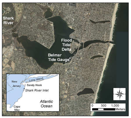
The CMS setup for Shark River Inlet provides is a succinct example for illustrating a number of methods and SMS tools that can be applied to most engineering projects. The area is characterized by being heavily structured, with a jettied inlet (and a jetty spur), developed bay shoreline (seawalls and riprap), and densely spaced groins, some of which on the south (up-drift) side have been notched. The overall goal of this guided example is to allow the user to work with real datasets, many of which were provided by the U.S. Army Corps of Engineers, New York District (NAN).
Goals for the exercise:
1. Assemble a base modeling grid
2. Set up specific features in the CMS
3. Develop several alternative grids
4. Compare calculated channel morphology change to measured channel morphology
The files and folders mentioned in this tutorial can be downloaded
Importing Bathymetric Datasets and Aerial Photographs
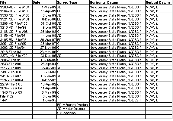
The original datasets put together for creating the Shark River Inlet grid are provided as a combined file that has already had the projection and datums modified. The original files include the bathymetry from a sampled (filtered) LIDAR dataset, a sampled multibeam survey of the north and south channels and back bay, Corps of Engineers channel surveys (NAN), and NOAA’s Coastal Relief Model (offshore bathymetry) . The final combined dataset includes all of the above listed datasets, and the full channel bathymetry collected by the NAN in 1999.
Table 1. NAN Surveys:
Open XYZ files and Viewing NAN Dataset
1. Open the Base.sms file located under Workshop/Initial,
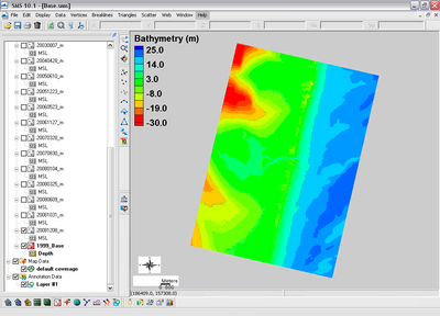
2. Select the Base - 1999_Base.h5 file to view the scatterset developed for Shark River Inlet. The SMS file may also be brought instead of the .h5 file to bring up all surveys (Figure 1). Note that all surveys have been converted to depths below msl and saved in the SMS .h5 binary format,
3. Click on Display, Display Options, or the button,
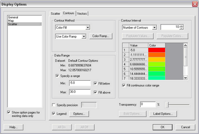
4. Go to the Scatter tab in the Scatter options, click to check the points off and contours on,
5. Go to the Contour tab, change contour method to Color Fill and adjust the data range as necessary (-5.0 to 30 m) (Figure 2).
Each dataset can be viewed separately by clicking on its name on the left side (the files stay separated in the SMS). If the points are checked, the selected set will display the points as the color you define in the display options, and all other datasets can be seen as a faded color. Setting the Transparency in the Contour Options allows for the background points to be visible in the SMS. The next step is to add a rectified aerial photographs for a background for aid in referring to location. There is an automated method for extracting a coarse aerial photograph or a navigation chart through SMS (Web, Import Web Imagery).
Add Rectified Aerial Photographs
1. Go to the Workshop/Image folder, drag the image (.tif) file over to the SMS window and drop where the plus sign appears by the pointer.
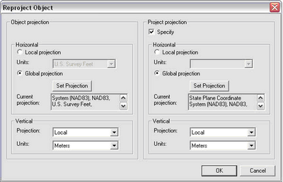
2. Rt-click on the image name and select Reproject and set from State Plane feet to State Plane meters (Figure 3. Note, that the Object Projection should be set to State Plane NJ in feet, and the Project Projection specified all in meters.),
3. Save the project into a new folder that you will work out of (File, Save As), and note that all files that are presently opened in the SMS will be rewritten to the new folder they are saved into.
Be sure to save the project before and after making major changes. If the original files are deleted after they are merged, it is a good idea to have copies of all important changes made to the datasets being modified.
CMS-Flow Setup
Grid Generation
For Shark River, the two grid options, constant and refined cell spacing, will run at more optimal speeds than a large project area such as a West Coast inlet or river mouth. Nevertheless, the refined option provides for more optimal CMS runtimes. The main inlet channel is the primary area of focus for capturing the correct current velocity with finer resolution, and should have 8-12 cells across it, limiting the cell size down to at least 10 m in the entrance channel. The two main back channels splitting off of the entrance, the north and south channel, also have large velocities (the north channel actually has the strongest current) and should be represented by at least several cells in width (minimum of 5 m in the narrow north channel).
Set Refine Points for Grid Generation
1. Click the Map Module button, or Map Data
2. Rt-click on default coverage, and under Type, Models, select CMS-Flow,
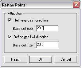
3. Click the Feature Point button to generate Refine Points, and place points in area of refinement, focusing on the end of the jetty tips and down the entrance channel (setting maybe 2 – 4 points) and with varying resolution with larger base cell sizes for the area near the back bay since that area does not need as fine of resolution for flooding and drying,
4. Click the Feature Point Selection button and select the generated point or points, Rt-click and click on Node Attributes (Figure 4), and set the base cell size for the area of the grid where the points are located.
5. The undo function does not yet exist in SMS, so be sure to save the project periodically (Save Project).
Next, the grid boundary is set square to the general orientation of the coastline, with the computational direction, I & J (or IJ triad), set according to the model type. For the CMS-Flow coverage (which was selected in step 2), the point of origin will be automatically placed in the lower left corner of the grid after the grid has been created. This is default for CMS-Flow. This means that for most Atlantic coast (east facing) projects the IJ triad will be located over land on the lower left corner. Do not change the direction of the IJ, because this is specific to CMS-Flow.
Generate the CMS-Flow Grid
1. Click the Create 2-D Grid Frame button
2. Draw two legs of the rectangular boundary for the model domain by clicking the lower-right ocean boundary corner point, then the upper ocean boundary corner, and then the upper landward boundary corner to close the box.
3. Use the Select 2-D Grid Frame button to select the center point of the purple outlined grid domain, adjust the edges by dragging the center point of each edge, and change the orientation by selecting the at the corner of the grid (Note that the IJ triad should be in the lower left corner),
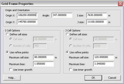
4. Rt-click the highlighted center button and click Properties to further modify the dimensions of the grid boundary (Figure 5),
5. Correct the angle orientation if it is far from 347º (the general orientation of the coastline is 13 deg from North), and set the I and J Cell Options to Use Refine Points and choose a maximum cell size and bias (cell size growth from refine points out), click OK,
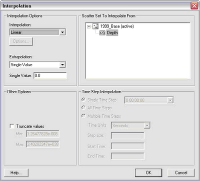
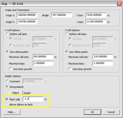
6. Click Feature Objects, Map 2D Grid, and check that all the grid properties are set properly, Use inner growth is turned off, the Interpolated Depth (Figure 6) from the merged file is selected, and define an elevation cutoff where cells will be non-computational land cells (always dry, act as a wall) (Figure 7), click OK.
Generating the first refined grid typically takes some trial and error testing to see how the grid looks. Be sure to modify the refine points to address areas of concern, particularly the number of cells across the entrance, north, and south channels, and groin cell width toward the lateral boundaries. Note that both the I and J directions do not need to be specified for each refine point, if refining only one direction is required.
Land-locked cells
After the grid is generated, two pop ups warn of overlapping cellstrings and land-locked ocean cells. These land-locked ocean cells that are not to be in the computation should be changed to inactive land cells. Also, the bay should be bound by land cells, and so any open ’ocean’ cells in the bay that lie on the grid boundary should similarly be changed to land cells.
To account for beach or berm cells to be wetted along the shoreline (cells with elevations higher than the land cell cutoff set in the grid generation section), sections of the beach should be changed to Active Ocean cells. This is difficult for Shark River because of the dense spacing of the groins as well as the fact that many of them are notched. Much of this information was retained in the LIDAR and subsequent generation of the bathymetric set provided for this example.

- Address Warnings: Fix Land-Locked Cells and Cellstring Warnings for the CMS-Flow Grid
1. For changing land-locked ocean cells to land cells, click the Select Grid Cell button if not already highlighted, and change the Z number to -1.0 (Figure 8), or manually select cells by dragging the mouse over the target ocean cells and change the Z,
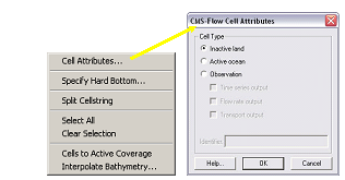
2. Rt-click on the cells, select Cell Attributes (Figure 9), and change the cell type from Active Ocean to Inactive Land cells, click OK,
3. The same process can be done for ocean cells that need to be changed to land cells along the bay edges (an aerial image will be useful for determining the proper widths of the channels); a simple way to check the entire land boundary is to use a directional selection method: hold down ctrl and click and drag the mouse along the outer edges of the landward side of the domain to highlight large sections,
4. To grab multiple areas, hold down shift while selecting new cells, and all will stay highlighted,
5. To change large sections of nearshore/beach cells that are land cells, select them with a polygon by clicking Edit, Select with Poly (clicking Crtl + Shift also initiates selecting by a polygon), and click a polygon covering a few cells across the ocean/land interface along a section of beach from groin to groin, and change to Active Ocean cells,
6. Change all required stretches of beach to ocean, and check that the landward grid boundaries have all inactive cells.
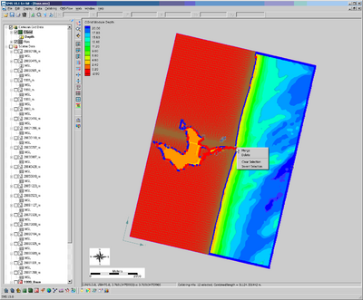
7. Select the Select Cellstring button and drag over the bay side of the grid to highlight the cellstrings generated there, and click delete (Figure 10),
8. Click Edit, Select All (Ctrl+A), and check to see if only the one ocean cellstring remains, delete all others.
As always, be sure to save the project to save the grid files, which are otherwise stored temporarily. Note that all files currently opened in the SMS will be saved over and may be recreated in the folder (with a 2 behind it).
If these steps are skipped, a grid is provided in the Workshop/CMS-Flow Grid\Initial Grid (1999Bathy) folder. Bring the *.cmcards file into the Base.sms project opened in SMS.
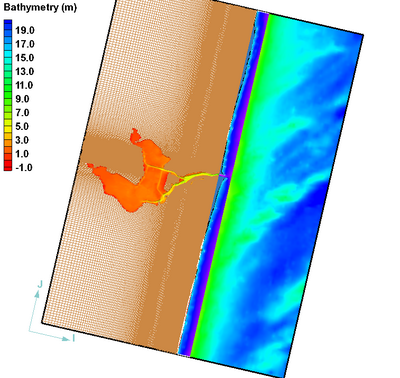
Bathymetry Preconditioning
Due to the nature of bathymetric data collection resulting in random data on the arbitrary day of the survey (as compared to the time frame of your project), certain areas of the grid may be poorly represented from scatter set triangulation and; therefore, from the final generation of the grid. It is necessary to smooth some features of the grid and leave other areas intact. Presently, there is one option to smoothing grid bathymetry, and that is based on a weighted average of 3x3 or 5x5 cells in a rectangular selection of the grid.
The triangulated nearshore bathymetry of Shark River is uneven in places, and the beach is the only area of concern for morphology change. The inlet, ebb delta, north and south channels, and offshore transverse shoals with considerable relief should be left as close to the original bathymetry as possible. There are two ways to approach smoothing sections of the nearshore, both using the 3x3 and 5x5 weighting scheme. One would be to select entire rows (J) of the grid and smooth everything, which would also smooth the channel somewhat, and would result in less control over the smoothing (Figure 11). The other is to smooth individual cells at a time
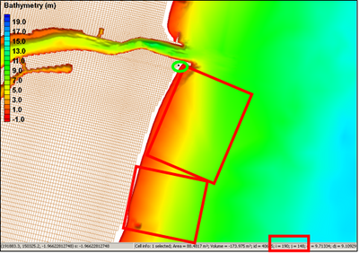
1. Determine the bounding cell id by looking at the corner cells (that make up the rectangular area defining the nearshore that is to be smoothed) by clicking the Select Grid Cell button and clicking on each cell individually, the I and J id is listed along the lower portion of the SMS window (Figure 12),
2. The I direction is that of the columns, and the J direction is that of the rows of the grid; record the I and J id of the bounding cells by step 1,
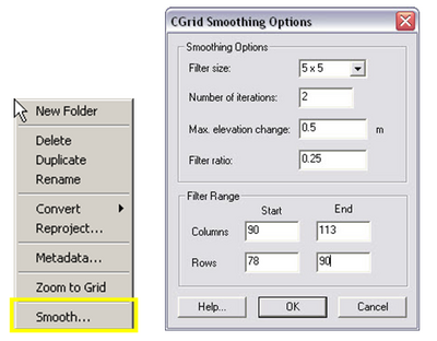
3. Rt-click the Cgrid under Cartesian Grid Data and click on Smooth (Figure 13) and the Cgrid Smoothing Options will pop up,
4. Set the Filter Size to 5x5, iterate twice, and leave Max. elevation changes, and filter ratio to the default, and change the column’s and row’s Start ID and End IDs to what the bounding cells were (figure 12), OK,
5. Check the area that was smoothed; repeat the process for the other stretch of nearshore bathymetry, preferably smoothing both the North Spit and South Spit nearshore.
Auxiliary Datasets
Other spatially variable, modifiable features for CMS-Flow include hardbottom (non-erodible levels), the D50 grain size, and the Manning’s n (bottom friction). Hardbottom is the level at which CMS is not allowed to erode the bottom further. It is automatically set to -999.0 (this is a negative depth for CMS, or otherwise a positive elevation) over all cells in the grid and that means that the cells are fully erodible. Setting these to the bed depth will prevent that bed from being eroded, but it can still be flooded, is computational, and will allow deposition. This is a useful tool for setting unusually or spuriously eroding cells in the model to hardbottom
CMS-Flow presently only simulates single variable D50 values, which can be spatially variable, for calculating initiation of transport, transport, and deposition. (Sediment mixtures will be added in a future CMS version.) The grid can interpolate a grain size scatterset if data are available for the area. Such data are not available for Shark River Inlet. However, changing the grain size to a larger value in the deep part of the entrance channel (where the channel thalweg is located) will suppress the erosion potential as it will require greater velocities to initiate sediment entrainment and represents channel armoring (fines winnowed away).
The option to modify the friction is useful for representing areas with restricted flow or with significant interference from structures. A good example of this at Shark River is the densely spaced bridge pilings for the three bridges spanning the main channels. Modifying the friction near the piling locations is one way to represent the impedance on flow around bridge pilings.
Hardbottom Dataset
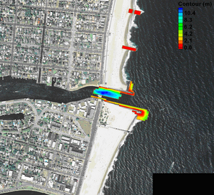
1. Modify the hardbottom cells by selecting Hardbottom under the Grid list of datasets. Click the Select Grid Cell button and clicking on each cell individually around the area of the main entrance channel thalweg,
2. Figure 14 shows what the hardbottom contours should look like after modifying them, Note that groins can also be changed to ocean cells but have modified hardbottom values (so that they cannot erode, but can receive accumulated sand),
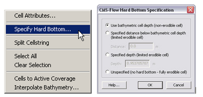
3. Rt-click on the selected cells, and select Specify Hardbottom, and then select Use bathymetric cell depth (non-erodible cell) (Figure 15), OK.
4. Save the progress of this grid by either saving the project again, or saving the grid only by clicking File, Save As, and choose the Save As Type as a CMS-Flow Simulation File (.cmcards).
D50 Dataset

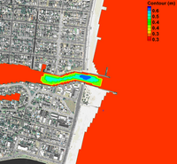
1. To modify the D50, select D50 under the Grid list of datasets. Click the Select Grid Cell button and click a polygon around the area of the main entrance channel thalweg,
2. Change the S value (Figure 16) from 0.26 mm (the SMS changes the decimal, but its close enough) to 0.40 and 0.50 mm similar to Figure 17,
3. Save the progress of this grid by either saving the project again, or saving the grid only by clicking File, Save As, and choose the Save As Type as a CMS-Flow Simulation File (.cmcards).
Manning N Dataset
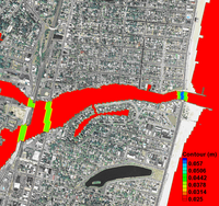
1. Next, modify the Manning’s n value from 0.25 to 0.3 underneath the locations of the bridges as shown in Figure 18,
2. Save the progress of this grid by either saving the project again, or saving the grid only by clicking File, Save As, and choose the Save As Type as a CMS-Flow Simulation File (.cmcards).
Boundary Conditions
The boundary conditions for CMS-Flow are assigned with cellstrings. When a CMS-Flow grid is generated, cellstrings are automatically generated along all of the boundaries. The user has the option to use any of these cellstrings or to create new cellstrings. In this case, all of the cellstrings may be deleted from the initial grid generation except the ocean cellstring. If all of the cellstrings are deleted, then the user must create the ocean cellstring by clicking at the start of the cellstring and double–clicking at the end of the cellstring. Note that the ocean cellstring should cover the whole offshore domain and therefore start and end at the land-ocean boundary.
For Shark River, there is little appreciable freshwater discharge, and so it is not included in the CMS simulation. The ocean boundary condition is set to the measured water surface elevations from Sandy Hook, verified with a tide gauge located inside the bay on the marine at the end of the South Channel. Data from the month of August 2009 are located in the folder Tide.
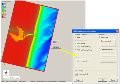
- Tidal Boundary Condition
1. Open one of the generated grids and select the Select a Cellstring button, rt-click the blue cellstring along the ocean boundary (if this cannot be selected it is because all cellstrings were deleted; this can be regenerated by clicking and clicking around the ocean cells or selecting Cellstring and Generate Along Boundary), select Assign BC (Figure 19),
2. Select the WSE-forcing boundary condition, and click curve undefined (Figure 19)
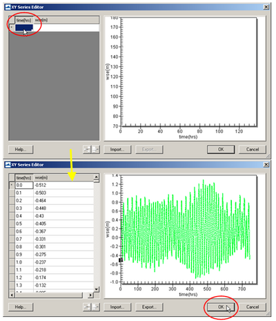
3. Open the excel file (SandHook_vs_Belmar.xls) in the Hands-on/Example 1 - Shark River Inlet/Tide folder, and select the time series in yellow for Sandy Hook with the time in hours on the left, and paste it into the XY Series Editor (Figure 20),
4. Zoom in on the graph on the right (Figure 20) to view the data up close,
5. Click export to save the xys (time series file) of the tide for use in other of the Shark River grid’s cellstrings, and save in the Tide folder, click OK when finished inspecting the pasted data, click OK.
6. Save the CMS-Flow Simulation File (.cmcards) in the original folder this alternative was saved in, and the new cellstring information will be saved with the card file.
Model Parameters
All of the CMS-Flow model parameters, settings, and output options are controlled from the CMS-Flow Model Control window. The window also has a section for Advanced Cards in which new features which have not been incorporated into the SMS interface yet or more advanced model features more experienced users.
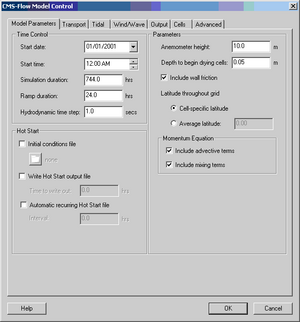
1. Click on CMS-Flow, Model Control, and set each tab as the following figures (Figures 21-25),
2. For Time Control, change the Simulation duration to 744.0 hours, Ramp to 24 hors, and Hydrodynamic time step to 1.0 (must be tested by running CMS-Flow only),
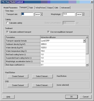
3. For Transport Parameters, change the Transport rate to 1.0 and the Morphologic time step to 10 seconds, check Use non-equilibrium transport and set the parameters as those in Figure 22,
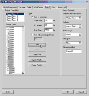
4. Set the time series output for the water surface elevation and velocity to the same output interval of 30 minutes, similar to Figure 23,by highlighting Output Times 1, setting the Start Time to 0.0 hr, Increment to 0.5 hr, and End Time to 744.0 hr, and clicking Add,
5. Set Output Times 2 for Morphology output at a 3-hr interval, by changing the Increment to 3.0 and adding, and selecting that on the drop down menu for Morphology,
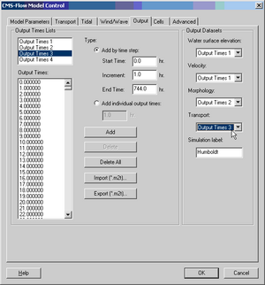
6. The same can be done for Transport, which should normally be set to an Increment on the order of the tide or wave time series (<3 hr; typically 0.5-1.5hr), and it is suggested that it be set to 1-hr output increment for Output Times 3 (Figure 24), OK.
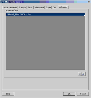
7. For the Advanced Tab, the option for using multiple threads or processors (in all caps, OPENMP_PROCESSORS 2.0) can be set up following Figure 36, OK.
CMS-Wave Setup
Grid Generation
Now that all modifications to the CMS-Flow grid alternatives have been finalized, the wave grid can be generated from the Flow grid. CMS-Wave grids are typically generated from scatter datasets, but can be a mirror image of the flow grid if the boundary condition (BC) locations are close enough to force both the tide and waves from the same BC area. In the near future, CMS will have the option to be run fully inline, where only one grid will contain all of the information needed to run both CMS-Wave and CMS-Flow.
The CMS-Wave IJ triad should be adjusted where the I-direction is pointing in the dominant wave direction, or more specifically from the open ocean. This means that it will be 180 deg off as compared to the CMS-Flow grid. Therefore, after the CMS-Flow grid is generated, the model domain should be set to include all major reaches of the bay, extending laterally a couple kilometers from the inlet and extending seaward well beyond the anticipated reach of the ebb jet. A good rule of thumb for setting the ocean boundary for inlet modeling is to place the boundary three or four times the length of the ebb jet (leaving provision for extreme discharges, such as during storm surge). The given bathymetry ends at approximately four times the length of the ebb jet at Shark River.

- Transforming the CMS-Flow grid to a CMS-Wave Grid
1. Open one of the generated grids rt-click the Grid in the SMS list, and click on Duplicate, select the copied grid (copy) to activate it, and go to Data, Switch Current Model (Figure 28),
2. Change the Model from CMS-Flow to CMS-Wave, click OK, and rename the grid by rt-clicking on the copy name and clicking Rename,

3. Set the jetty and groin cells to rubble-mound type structures by selecting the cells (Figure 27), and rt-click, Cell Attributes.., and select a Rubble-mound from the Structure Type, click OK.
4. File, Save As, Wave.sim (selecting the Save As Type as a .sim for simulation) in the folder with the CMS-Flow grid.
Providing Ocean Buoy Data to CMS-Wave
After all modifications to the CMS-Wave grid are complete, the spectral waves or wave parameters can be generated for the wave grid. Full (directional) spectra can be imported into the SMS for the CMS-Wave, as well as simplified wave parameters (angle, wave height, and period, etc). Directional spectral data collected by the National Data Buoy Center (NDBC) or Coastal Data Information Program (CDIP) buoys, available from the National Oceanographic Data Center, can be processed (transformed to the model domain) and used as a source for wave input to CMS-Wave.
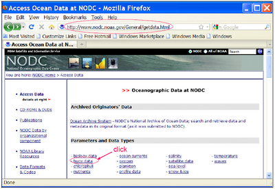
Importing NDBC bouy data
- Run ndbc-spectra.exe to read the NDBC standard directional wave file and prepare the CMS-Wave input spectral *.eng file.
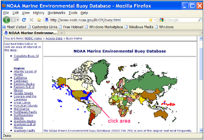
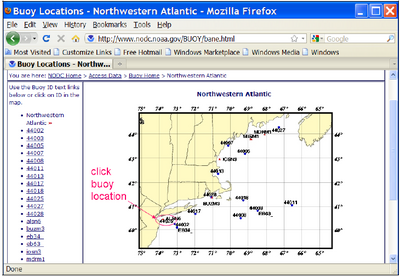
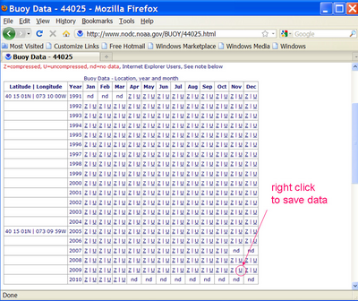
1. Download the NDBC standard monthly directional wave spectral file from
(e.g., 44025_200912) (Figures 28 to 31), this is provided under Hands On Materials - Shark River Inlet/Waves.
2. In the DOS mode (Command Prompt), run ndbc-spectra.exe (Figure 32),
3. Responding to the on-screen input, type the NDBC spectral filename,
4. Type the starting time stamp (default value is 0) for saving output file(s),
5. Type ending time stamp (default is 99999999) for saving output file(s),
6. Type the time interval (hr) for saving output data,
7. Type 2 to save the CMS-Wave *.eng and *.txt files,
8. Type the local shoreline orientation (actually the CMS-Wave grid y axis) in Polar Coordinates (deg, positive from North covering the sea, e.g., 180 deg for a north-south oriented project on the Atlantic coast),
9. Type the NDBC buoy location water depth (m) and then the CMS-Wave seaward boundary mean water depth (m), e.g. Buoy 44025 has a nominal depth of 36.3 m,
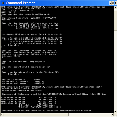
10. Type 1 to include wind or 0 to skip the wind, and to complete the run (Figure 32),
The fort.15 and fort.18 files are the parameter and spectra, respectively, to be imported in to CMS-Wave. Two additional files are generated: fort.12 and fort.19, which are the tabulated wave (and wind) parameters for the full-plane and half-plane wave propagation coverage, respectively. Matlab fig1set.m and fig2sets.m can read these files to plot the wave and wind data time series.
11. Rename fort.15 to *.txt and fort.18 to *.eng (half-plane wave energy), which was renamed to wave_shark_2009.eng,
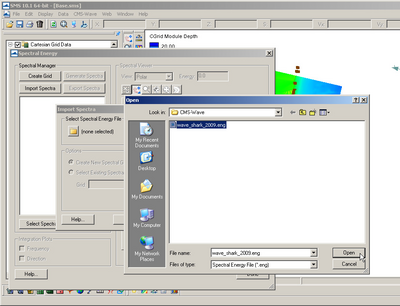
12. In SMS, go to CMS-Wave, then Spectral Energy, and select Import, and select the *.eng file just created (Figure 33),
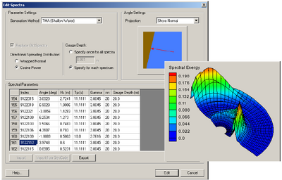
13. Save as a new CMS-Wave file (.sim) and all necessary files including the spectral energy file will be saved with that name (Figure 34).
If these steps (from pages 27-31) are skipped, there is a grid provided under Hands On Materials - Shark River Inlet/CMS-Wave that has the spectra included.
Importing CDIP buoy data
Importing CDIP buoy data is similar to the method of importing NDBC buoy data.
1. Download the CDIP wave file ?nav=historic&sub=data (e.g., sp154-200912) (Figures 35 to 37), also provided under Hands On Materials - Shark River Inlet/Waves,
Note that the only difference is the processed CDIP wave spectra do not need to be transformed to the CMS-Wave seaward boundary. The data can be directly input to CMS-Wave. Examples given are CDIP 154 and NDBC 44025 standard spectral files for Dec 2009.
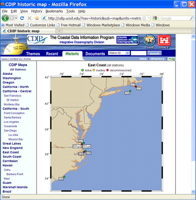
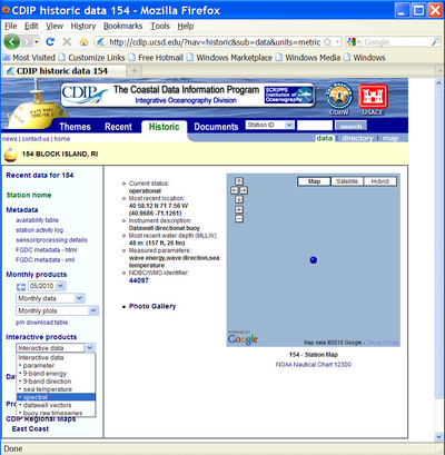
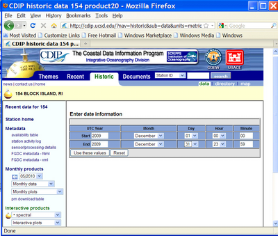
2. Run cdip-spectra.exe and follow the same steps as those from pages 30-31 (from processing the NDBC buoy data with the ndbc-spectra.exe program), to read the CDIP standard directional wave file and prepare the data for input to CMS-Wave as a *.eng file.
Model Control

To setup the model parameters for CMS-Wave:
1. Go to CMS-Wave, Model Control, and turn on Allow wetting and drying and Bed friction (Figure 38),
2. Users can also specify constant or varied forward and backward reflection coefficients in Settings,
3. Water level and wind information are optional source as specified under Wave Source in addition to the spectral input data,
4. File, Save As, Wave.sim (selecting the Save As Type as
Steering
Steering is the coupling process between CMS-Flow and CMS-Wave. In CMS-Flow versions v3.75 and older (explicit CMS-Flow), the steering was done by the SMS interface. The new inline CMS (implicit CMS-Flow) contains both CMS-Flow and CMS-Wave and performs the coupling process internally. Therefore, depending on what version of CMS-Flow wants to run, the steering process is slightly different.
Before running steering, it is a good idea to test the CMS-Flow and CMS-Wave separately to make sure there are no problems with their grids, or input parameters. Once the CMS-Flow and CMS-Wave models have been setup properly and loaded in SMS, the steering can be initiated.
CMS-Flow (V3.75 and older) and CMS-Wave
Note that the input spectra need to be spaced at regular time intervals and begin at the same time as the CMS-Flow model.
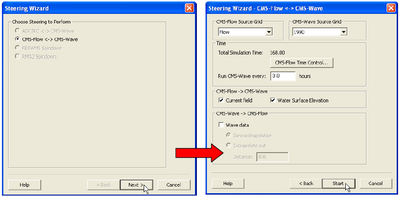
- Start Steering Module to run the CMS
1. Be sure to save the flow and wave grids into the same folder,
2. Open the SMS Steering Wizard by clicking on the menu Data | Steering Module.
3. Click on CMS-Flow <-> CMS-Wave, click next, and set as the following Figure 30, click Start.
CMS-Flow (V4.0 and newer) and CMS-Wave
CMS Versions 4.0 and newer the steering process is done internally by the CMS. This means that that both CMS-Flow and CMS-Wave are contained within a single code or executable. Currently, this inline version of CMS only contains the implicit CMS-Flow. Therefore, if the user decides to switch from explicit to implicit solvers, the user must also change the CMS-Flow executable under the SMS preferences. To run the inline CMS in steering, the user must specify the steering options in the advanced cards and then execute the CMS-Flow from the SMS interface.
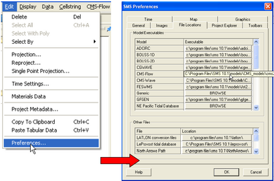
- Change the CMS-Flow executable to the inline code (see Figure 40).
1. Click on Edit | Preferences.
2. Under Model Executables change the name of the executable for CMS-Flow to the name of the executable provided in the DVD. The executable name should be something like CMS_2D_v4p0.exe.
The next step is to provide the steering information using the advanced cards. Note that when running the inline CMS the couling between CMS-Flow and CMS-Wave is set to full. This means that both the water level and currents are passed from CMS-Flow to CMS-Wave and all of the wave information is passed from CMS-Wave to CMS-Flow. The information that needs to be provided is the steering interval, which is the time interval on which the CMS-Wave model is run and should also correspond with the time interval between input spectra. Note that the input spectra need to be spaced at regular time intervals and begin at the same time as the CMS-Flow model. The steering interval is provided in units of hours.
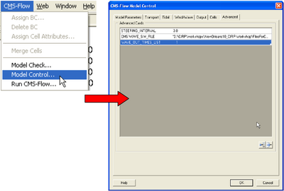
- Set the steering information (See Figure 41)
1. Click on CMS-Flow | Model Control…
2. . Enter the steering interval and CMS-Wave *.sim file using the cards shown in Figure 41. Note that the full path to the *.sim file must be provided within quotation marks.
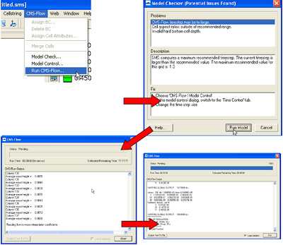
- Start Steering Module to run the CMS (see Figure 42)
1. Load the CMS-Flow project
2. Click on CMS-Flow | Run CMS-Flow.
3. When the model is finished, click on exit
The inline code will produce two files named Intpcoef_flwav.bin, and Intpcoef_wavfl.bin. These files contain the interpolation information between the CMS-Flow and CMS-Wave grids. If the model is restarted the model will automatically detect these files and read them.
Viewing Results and Making Animations
Once completing the CMS simulations, animations may be generated to view the current, wave, or sediment transport results. In order to view the simulation results a time series plot must be available in the dialog box on the left, and a contour plot for a calculated variable (scalar or vector) displayed in the graphics window. SMS provides a handy tool to perform this task.
Load the solution file
1. Choose File | Open,
2. Browse your folders to find the solution file, ETD1999_sol.h5 (under Hands On Materials - Shark River Inlet/Simulations),
3. Select ETD1999.cmcards,
4. Press Open.

Plotting bathymetry contours
1. Choose Display | Display Option, Select the Cartesian Grid on the left hand side of the Display Options window (Figure 43),
2. Check the boxes for the Contours and Grid Boundary, and uncheck the Hard bottom symbols and Cellstrings,
3. Select the Contours tab at the top of dialog (Figure 44), and choose the Contour Method | Color Fill, click the Color Ramp button to adjust the color scheme, set the proper depth range by checking the Specify a range (0-20 m), and change the Contour interval to 11, plot depth contours every 2 m,
4. Click the Options next to the Legend to select font for the contour label.
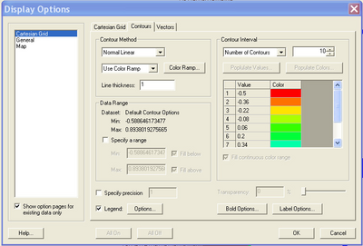
Generating a Contour Plot
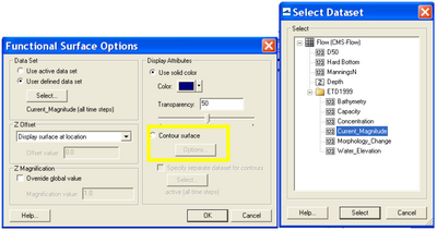
- Generating contour plot of current magnitude on top of depth contour
1. Check the box for the Functional surface, and click the Options below it, Select User defined data set under Data Set in the dialog (Figure 43),
2. Highlight Current_Magnitude and click the Select button, choose the Z Offset | Display surface with user defined offset,
3. Click the Contour Surface button and the Options below it to set up contour options (repeat steps 4-8 in the Plotting Bathymetry Contours, (Figures 43-44).
Making an Animation
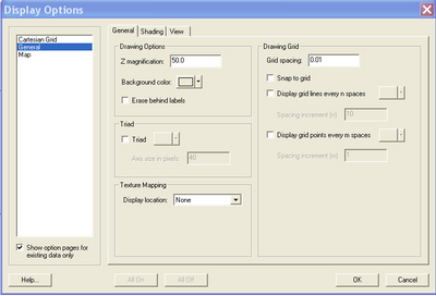
- Generating oblique view of the contour plot
1. Select the General on the left hand side of the Display Options window (Figure 46),
2. Set Z magnification under the General | Drawing Options button to 50 (Figure 46),
3. Click the Rotate tool, and rt-click and hold the button to adjust viewing angle of the plot.
Saving an animation file

1. Choose Data | Film Loop (Figure 47), check the box for the Create AVI File, name the animation file, and go the Next,
2. Set up animation time and click the Next, click the Clock Options button and select the style and location of the time bar,
3. Click the Finish button and start to save the AVI file.
Alternative Grids and Other Functions
Creating Alternative Grids
Testing various CMS grids developed with varying cell sizes and can result in several grid generations, so be sure to clearly label each saved grid with some note of metadata information describing what is contained in the grid setup. Metadata can be entered through the SMS interface by right-clicking on a dataset and entering the information.
In addition to varying grids, the practical use of the CMS lies in variations of "engineered modifications" (alternatives). Some modifications can be anything from modified bathymetry (using different surveys), to changing a structures configuration, to modifying any of the CMS-Flow spatially variable parameters discussed in the previous section. The result of this process of alternative grid generation can be complicated; therefore, be sure to clearly label grids and place them in labeled folders or subfolders.
One of the reasons the 1999 bathymetry of Shark River was provided for this example was to use a deeper bathymetry from a year where shoaling had not begun at Shark River Inlet (beginning in the early 2000s because of nourishment of the adjacent beaches). The scattersets of surveyed channel bathymetry can be interpolated onto the grid and saved as a new grid alternative.
Modifying a Section of the Grid Bathymetry
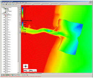
1. Following saving the grid in a new location with a changed title (save the cms-flow file as a .cmcards), zoom in to the inlet on the grid and select the Select Grid Cell button
2. Highlight the area of the channel (using select with a polygon) where a scatterset can be interpolated from, (it is recommended that a recent survey be used to cover a larger area as shown in Figure 48),
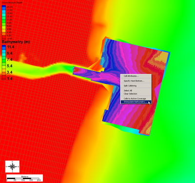
3. Rt-click and select Interpolate Bathymetry, and choose the dataset that will be interpolated into the grid (Figure 49),
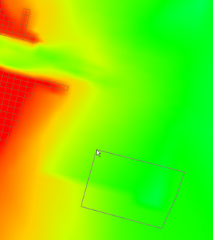
4. After the bathymetry is interpolated, there may be uneven areas at the edges (for projects where interpolated datasets are greatly different it is suggested that a new grid be generated from the merged scattersets), and smoothing sections of the edges is an option (Figure 50),
5. Save the grid as a new CMS-Flow Simulation File (.cmcards).
Modify the Jetties
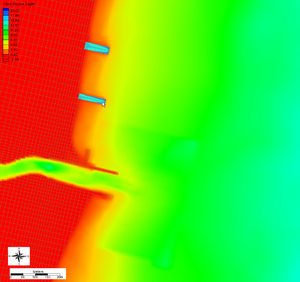
1. Open the original grid with the saved grid modifications (D50, Mannings n, etc.) and save the grid in a new location with a changed title, e.g. jetty_length, (save the cms-flow file as a .cmcards), zoom in to the inlet on the grid and select the Select Grid Cell button,
2. Highlight the cells oceanward of the North Jetty (holding the Ctrl button down) out 100 m from the present extent, rt-click and modify the cells to land cells, and change the Z values to -1.5m,
3. Highlight the ocean cells of the groin notches so that the entire groin is closed, rt-click and modify the cells to land cells, and change the Z values to -1.5m (Figure 22).
4. Save the grid as a new CMS-Flow Simulation File (.cmcards).
Adding a Channel Configuration
Some GIS data can be read into the SMS such as shapefiles or raster images. Presently, CAD and Microstation drawing files cannot be imported; however, a drawing that is converted to a shapefile can be brought into the SMS.
1. In the Workshop/Channel folder where several shapefiles have been placed, and drag in all three shapefiles (.shp) over to the SMS window,
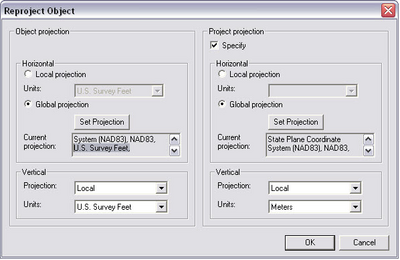
2. These will be displayed in State Plane New Jersey in feet and must be reprojected to meters, rt-click on each file and Reproject each from feet to meters (Figure 52), uncheck all but the Channel.shp, and use the button to highlight the shapefile,
3. Convert this into map features by clicking on Mapping, Shapes to Feature Objects, and if a popup prompts that the shapefiles are not highlighted and whether or not to "Use all shapes in all visible shapefiles for mapping?" (make sure these are all turned on), click no and go back and select only one shapefile at a time, otherwise click through the prompt to convert to Feature objects,
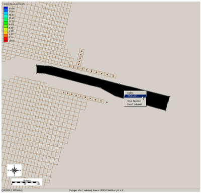
4. Click on Map Data on the left or the Map Module button, and select the Create Feature Arc tool, and connect the missing arc features of the channel outline (Figure 53), Select all arcs, and click on Feature Objects, and Create Arc Group, and the polygon will be fixed
5. A new tool should now be available, the Select Feature Arc Group, select the arc and go to Feature Objects, and click i, and click OK, and again go to Feature Objects, and click Build Polygons,
6. Another new tool should now be available, the Select Feature Polygon , use this to highlight the polygon inside the arcs, and click Attriubutes, and select either Land or Ocean,
7. Open Display Options , and under the map tab check the Polygon box, here colors can be assigned to the label Land or Ocean, OK,
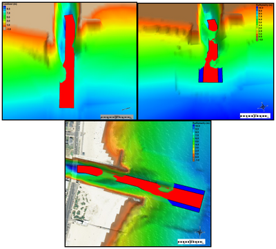
8. Selecting the polygon arcs with the button, the Z can be modified for the arcs to allow viewing the polygon as a plane within the 3-D visualization (Figure 54).
Post Processing
The results of the CMS calculated morphology change can be visualized several ways, from three dimensional or planar view of the bathymetry, planar view of the volumetric erosion and accretion, and with 1-D cross-sections of the time series. All vector and scalar information can be extracted from points and arcs (and polygons) in SMS. This section will cover the methodology used to post process time series morphology change data.
Calculating Channel Infilling
To plot channel infilling in SMS in a graphical format, the results in the solution file need to be changed from depths (the depth below the datum in which CMS calculates) to elevations.
Change Depth to Elevation
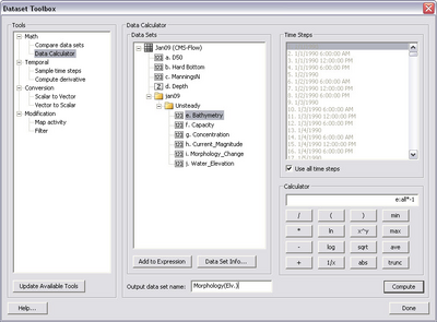
1. Load the SMS file run1.sms (and solution file, if it does not load automatically) located in the directory Hands-on/Alt1 Solutions/Run 1,
2. Rt-click on the Time Series window on the left and select "Time Settings", and change the time reference from Relative to Absolute,
3. In the Cartesian Grid Module, click Data, Data Calculator, and the Data Calculator should be selected in the Tools section as shown in Figure 55,
4. Select the Bathymetry scalar dataset, under Time Steps check the Use all time steps on, and double-click the Bathymetry (highlighted in Figure 55),
6. The line under Calculator will display e:all, add the multiplication symbol (*) and negative 1 (-1) as shown in Figure 55,
7. Change the Output data set name similarly to Figure 55 so as to distinguish this dataset from the original Bathymetry output, click Compute, and after the scalar set appears in the SMS window (Figure 55), click Done. (Note: values for the contours may need to be adjusted to view elevation range.)
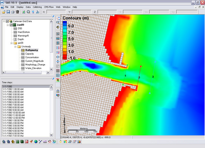
Create Feature Arcs for Extracting Time Series Morphology Change
The next step is to generate the cross sections, or arcs, in SMS to extract data with.
1. Click the Map Module button, or Map Data,
2. Rt-click on default coverage, and under Type, Generic, Observation,
3. Click the Create a Feature Arc button to generate the arcs that cross sections will be extracted from, and click on one side of the channel and double-click on the other side to close the arc,
4. Click the Select a Feature Arc button and select the generated arc (Note that there is a direction associated with the arc, which determines the sideview of the cross section),
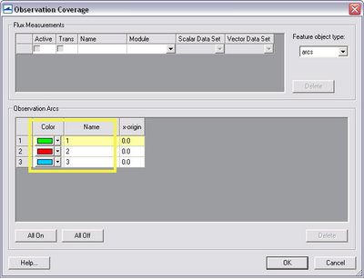
5. Rt-click and click on Attributes, and set the color and name(s) of each arc which are listed together in the Observation Coverage options (Figure 57), click OK.
Plotting Time Series Morphology Change in SMS
The following step is the final step for generating the graph in SMS. This is also the present method to extract and export this information in text format for use in other plotting software.
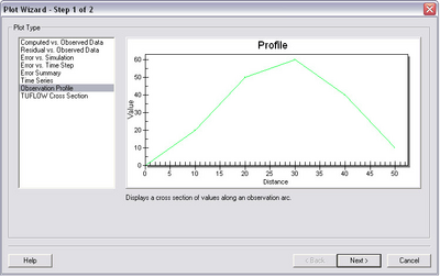
1. Click Display, Plot Wizard, and click Observation Profile (which should have the display in Figure 58 and Next should be available if the arcs were generated in the Observation Type Coverage in the above Create an Arc section), click Next,
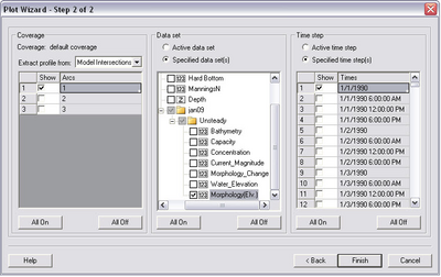
2. Following Figure 59, under Coverage check one arc (though multiple can be plotted), under Data set select Specified data set(s) and select the generated Morphology (Elev.) set only, and under Time step select Specified time step(s) and check on several times spaced apart by at least several days to months, click Finish,
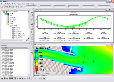
3. Rt-click on the plot (Figure 60) and select view values.., and a table will appear with all the plotted distance and elevations given in the graph, (Note this ascii table can be copied and pasted into excel),
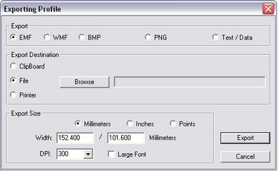
4. To export the data in different formats, rt-click on the plot, and select Export/Print for several options to export the graph or data from the graph (Figure 61),
5. To add more profiles or time-series, rt-click on the plot, and select Plot data.. to bring up the original options from Figure 61.
Calculating Sediment Transport Rates and Budgets with the CMS
Calculating accurate sediment transport rates is necessary for predicting channeling infilling, inlet and nearshore morphology change, and on a more basic level understanding sediment pathways and formulating sediment budgets. In the CMS, sediment transport statistics are calculated across predefined lines or polygons defined by feature arcs and polygons in a post-processing procedure. The total-load sediment transport rates calculated from CMS-Flow are integrated across user-defined boundaries. The sediment transport statistics are calculated from the integrated sediment transport rate. The calculated statistics are the net, gross, positive and negative total-load sediment transport rates and are output in units of either cy/ft or m3/m.
Loading Solution and Creating Obervation Arcs

1. Load the Shark River Inlet-Workshop__Alt 1.cmcards into SMS by dragging it into the SMS or by clicking File | Open | Shark River Inlet-Workshop__Alt1.cmcards. The solution file should load in automatically.
In the project explorer to the left of the SMS window, either change the type of the Map coverage to Observation or create a new Map coverage of type Observation.
2. Specify an Map Coverage of type Observation by either changing the type of a current Map Coverage or creating a new Map Coverage
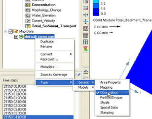
- a. To change the type of a current 'Map coverage Right-click on the default coverage and select Type | Generic | Observation
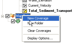
- b. To create a new Map coverage, right-click on Map Data in the project explorer, then select New Coverage
3. Change the name of the Observation Map Coverage to Alt 1_Obs_Arcs.

4. Create feature arcs and polygons. Make sure you are in the Map module by clicking on the Map Module Tool or by clicking on Map Data (Figure 65). The Map Module toolbar should become available in the SMS window.
5. Click on the Create Feature Arc tool.
6. Click on the starting and ending points on the grid that define the transect for calculating the sediment transport statistics.
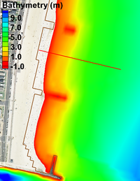
An example of a Feature Arc for calculating the longshore sediment transport at Shark River Inlet is shown in Figure 66. In the case of longshore transport, the feature should extend beyond the breaker zone and closure depth to capture all, mainly, wave-induced longshore sediment transport. Make sure the arc does not touch inactive land cells as this may cause interpolation problems in the SMS.
The positive direction of the sediment transport is defined by the Feature Arcs direction. To view the arc direction, click on the Select Feature Arc tool and right-click on the Feature Arc once.
The arrows displayed at the beginning and end of the transect indicate the direction of the arc which defines the positive for all fluxes or vectors calculated across it.
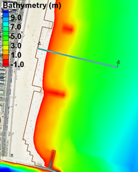
If necessary, the arc direction may be changed by clicking on the Select Feature Arc tool, and selecting the feature arc by right-clicking it once and selecting the option: Reverse Arc Direction. The same applies for feature polygons.
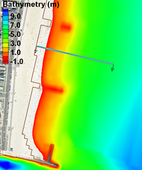
Creating "Ones" Dataset

The sediment transport calculation across a feature arc requires a dataset of the same size and length and constant value of one. To create this dataset:
1. Select the Cartesian Grid Module
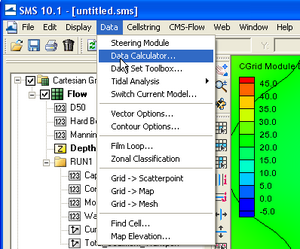
2. Click on Data | Data Calculator.
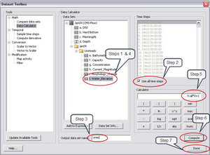
3. Select the water elevation dataset.
4. Click on the Use all time steps checkbox.
5. Change the name of the output dataset to ones.
6. Double-click on the water elevation dataset so that it appears in the Calculator.
7. In the Calculator, multiply the dataset by zero and then add one.
8. Click on Compute. The calculation might take a few minutes if the dataset is large. Once the calculation is completed, the output dataset will appear under the Datasets window.
9. Click on Done to exit the window.
Sediment Transport Integration
To obtain the sediment transport statistics, the sediment transport is first integrated spatially to compute a time series of sediment transport across the Feature Arc. This procedure in done in the SMS Plot Wizard. The sediment transport vector field is interpolated to the points where the arc intercepts cell faces and is then integrated across the Feature Arc. Follow each step outlined below:
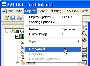
1. Open the Plot Wizard by clicking on Display | Plot Wizard

or clicking on the Plot Wizard icon
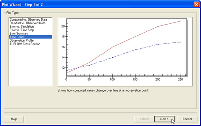
2. In the Plot Wizard – Step 1 of 2 window, select Time series as the Plot Type and then click Next>.
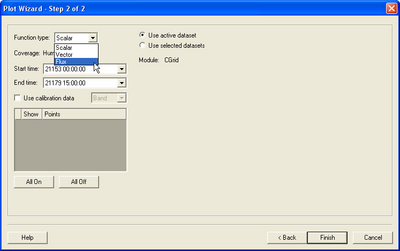
3. In the Plot Wizard – Step 2 of 2 window, select Flux as the function type.
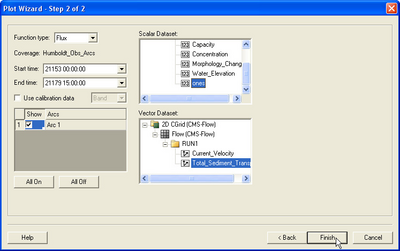
4. Click on the feature arc checkbox. Select the ones dataset for the scalar dataset, and the sediment transport as the vector dataset. Make sure the start and end times are correct. Click Finish.
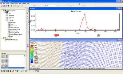
The computation might take a few minutes, especially if the dataset is large.
Calculating Sediment Transport Statistics
There are two ways of calculating the sediment transport statistics. One is with a Fortran executable, and the other is with an Excel spreadsheet. A simple Fortran executable is provided that calculates the transport statistics based on a time series of integrated (along arc) transport rates obtained in the previous section. The program can be run from a command prompt, a script file or by simply double clicking on the executable and providing the name of the input file.
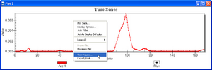
1. Right-click on the time series plot and select View values…

A table will be displayed with the time in hours and integrated sediment transport rate across the feature arc.

2. From the View Values window, select the data from the data and copy-paste it to a text editor such as Wordpad. Note the number of rows in the dataset by looking at the id number of the last row in the View Values window. Save the file with the extension *.txt (see Figure 80). The data may also be saved as an *.xys file (SMS xy seris file). In this case, the file needs a header as shown in Figure 80, where the second entry is a file id, the third entry is the number of time steps, and the last entry is a name for the time series.
2. Double click on the executable named proc_flux.exe. The executable does not need to be in the same folder as the input file. If the file is not in the same directory, the path should be specified before the file name. If the path contains spaces quotation marks should be used.
3. Press enter when the executable is finished.
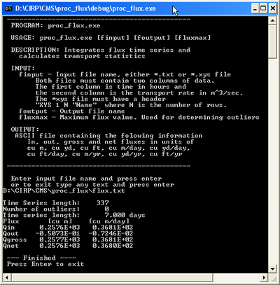
An example of the command prompt showing the steps for calculating the sediment transport statistics with the proc_flux.exe application is shown in Fig 81.

If no output file is specified, the default output file name is Flux_statistics.txt. An example of the output file is shown in Fig 82.