JALBTCX/QRStep3: Difference between revisions
(Created page with "{{DISPLAYTITLE:Quick Response Toolbox: Step 3 - Generate Difference Grid by Clip Mask}} File:QR Step3.jpg|thumb|right|alt=A screenshot of the ArcPro geoprocessing panel for Step 3. The "Before Raster(s)" and "After Raster(s)" allow the user to select the inputs from a drop down menu or the file explorer. "Before Raster Label" and "After Raster Label" are text inputs (strings). The "Clip Mask" and "Output Geodatabase" allow the user to enter file locations as text or se...") |
No edit summary |
||
| Line 1: | Line 1: | ||
{{DISPLAYTITLE:Quick Response Toolbox: Step 3 - Generate Difference Grid by Clip Mask}} | {{DISPLAYTITLE:Quick Response Toolbox: Step 3 - Generate Difference Grid by Clip Mask}} | ||
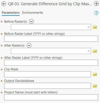
[[File:QR Step3.jpg|thumb|right|alt=A screenshot of the ArcPro geoprocessing panel for Step 3. The "Before Raster(s)" and "After Raster(s)" allow the user to select the inputs from a drop down menu or the file explorer. "Before Raster Label" and "After Raster Label" are text inputs (strings). The "Clip Mask" and "Output Geodatabase" allow the user to enter file locations as text or select from the file explorer. The "Project Name" input is a text input which must start with letters.|Figure 5: Step 3 - Generate Difference Grid by Clip Mask. Red stars indicate required fields.]] | [[File:QR Step3.jpg|thumb|right|alt=A screenshot of the ArcPro geoprocessing panel for Step 3. The "Before Raster(s)" and "After Raster(s)" allow the user to select the inputs from a drop down menu or the file explorer. "Before Raster Label" and "After Raster Label" are text inputs (strings). The "Clip Mask" and "Output Geodatabase" allow the user to enter file locations as text or select from the file explorer. The "Project Name" input is a text input which must start with letters.|Figure 5: Step 3 - Generate Difference Grid by Clip Mask. Red stars indicate required fields.|343x343px]] | ||
'''Summary:''' This step uses raster math to create a “Difference Grid”. First, elevation surfaces are created for each year of data using the clip mask. The script then uses arcpy.sa.Minus to get the difference grid between two input rasters. The output raster cell size is determined by default based on the cell size of the input raster with the smallest cells. For example, if a DEM raster with a 1m resolution is subtracted by a DEM raster with a 3m resolution, the output will be a 1m raster. The outputs of this step include surface grids and a difference grid to be used in subsequent steps for volume change. | '''Summary:''' This step uses raster math to create a “Difference Grid”. First, elevation surfaces are created for each year of data using the clip mask. The script then uses arcpy.sa.Minus to get the difference grid between two input rasters. The output raster cell size is determined by default based on the cell size of the input raster with the smallest cells. For example, if a DEM raster with a 1m resolution is subtracted by a DEM raster with a 3m resolution, the output will be a 1m raster. The outputs of this step include surface grids and a difference grid to be used in subsequent steps for volume change. | ||
| Line 22: | Line 22: | ||
Figure 6 displays displays surface and difference Grids for Homer, AK example data. Figure 6A: 2018 surface grid, 6B: 2019 surface grid. 6C: Difference grid between 2018 and 2019. | Figure 6 displays displays surface and difference Grids for Homer, AK example data. Figure 6A: 2018 surface grid, 6B: 2019 surface grid. 6C: Difference grid between 2018 and 2019. | ||
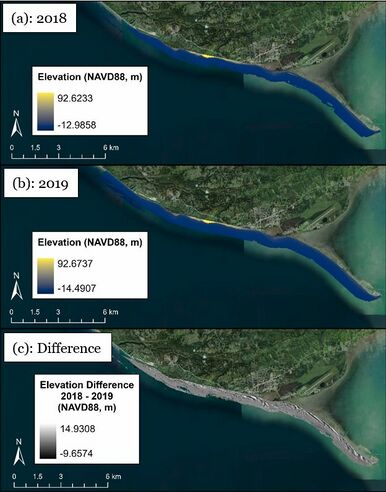
[[File:QRFigure6.jpg|thumb|center|alt=The surface rasters for both 2018 (A) and 2019 (B) are shown with elevations, in NAVD88, visualized from blue to yellow. The extent of both rasters is identical as the tool has only selected cells where both datasets are not null. Bellow those the difference raster (C) is shown with elevation difference, in NAVD88, shown from black to white. Areas along the coast show a high variability in difference results.|Figure 6: Surface (a & b) and Difference Grid (c) outputs from Step 3 in Homer AK.]] | [[File:QRFigure6.jpg|thumb|center|alt=The surface rasters for both 2018 (A) and 2019 (B) are shown with elevations, in NAVD88, visualized from blue to yellow. The extent of both rasters is identical as the tool has only selected cells where both datasets are not null. Bellow those the difference raster (C) is shown with elevation difference, in NAVD88, shown from black to white. Areas along the coast show a high variability in difference results.|Figure 6: Surface (a & b) and Difference Grid (c) outputs from Step 3 in Homer AK.|492x492px]] | ||
==Useful Links== | ==Useful Links== | ||
[[JALBTCX|JALBTCX Main Documentation Page]] | [[JALBTCX|JALBTCX Main Documentation Page]] | ||
Refences: Quick Response Toolbox | |||
Revision as of 22:14, 9 December 2024
Summary: This step uses raster math to create a “Difference Grid”. First, elevation surfaces are created for each year of data using the clip mask. The script then uses arcpy.sa.Minus to get the difference grid between two input rasters. The output raster cell size is determined by default based on the cell size of the input raster with the smallest cells. For example, if a DEM raster with a 1m resolution is subtracted by a DEM raster with a 3m resolution, the output will be a 1m raster. The outputs of this step include surface grids and a difference grid to be used in subsequent steps for volume change.
Before Raster(s): Raster from the earlier point in time
Before Raster Label (YYYY or other strings): Desired label for the before raster. The year is suggested but the user is free to decide.
After Raster(s): Raster from the later point in time.
After Raster Label (YYYY or other strings): Desired label for the after raster. The year is suggested but the user is free to decide.
Clip Mask: Clip Mask generated in Step 2.
Output Geodatabase: Full file path, including name and file extension, for desired output geodatabase.
Project Name (must start with letters): Desired name for the project. The output file name will be “User-defined project name” + “_’Type of Grid’_” + “before year” + “after year”. This tool will output: one before raster grid per segment, one after raster per segment and one difference grid per segment.
Best Practices & Example Data:
Figure 6 displays displays surface and difference Grids for Homer, AK example data. Figure 6A: 2018 surface grid, 6B: 2019 surface grid. 6C: Difference grid between 2018 and 2019.
Useful Links
JALBTCX Main Documentation Page
Refences: Quick Response Toolbox

