Filter1d: Difference between revisions
| Line 180: | Line 180: | ||
==Appendix A== | ==Appendix A== | ||
The sinc function is calculated as | The sinc function is calculated as | ||
{{Equation| <math> r(i)= \frac{\sin{i \pi f_c}}{i \pi} </math>|2=1}} | {{Equation| <math> r(i)= \frac{\sin{i \pi f_c}}{i \pi} </math>|2=1}} | ||
where | where <math>f_c </math> is the cut-off frequency. The following windows are available in Filter1D: | ||
is the cut-off frequency | |||
|} | * Hanning | ||
{{Equation| <math> w(i)=1/2(1-\cos{2\pii/N}) </math>|2=2}} | |||
Revision as of 20:45, 9 September 2010
Filter1D - Time Series Analysis Tool
By Alejandro Sánchez
Purpose
The Coastal Inlets Research Program Technical Wiki herein describes a desktop computer program for filtering and preprocessing time series in support of numerical modeling applications. The utility is the first time series analysis tool to be incorporated in the Surface Modeling System (SMS). The graphical user interface is designed to be extremely easy to use.
Introduction
Preprocessing and quality control of input time series for surface water flow and sediment transport numerical models are key steps in setting up the simulations and obtaining correct results. In the past, users of the SMS have performed these tasks using external software such as MATLAB® or EXCEL® and required several steps. The software presented herein, provides users of the SMS, a one-stop package for preparing model input time series and allows users to interpolate, resample, filter, and transform any type of model forcing and supports SMS compatible file formats for ease of data transfer.
The main feature of the software is the ability to apply high-pass, low-pass, band-pass, and band-stop filters to time series. There are many types of filters available, and each have their own advantages and disadvantages. Filter1D uses a windowed sinc filter which is a non-recursive finite impulse response filter. Non-recursive filters consist of convolving the input time series with a weight function and therefore only depend on the non-filtered points. Recursive filters use neighboring filtered points and therefore require stepping or iterations. The advantage non-recursive filters compared to recursive filters is that they are more stable and mathematically simpler. Their disadvantage is that they may require a large number of weights to achieve a desired filter response (amplitude reduction in frequency domain). If the weights are symmetric, then an equal weight is given to points to the left and to the right of a given point and the filter is said to be symmetric and therefore produces no phase lag. For details on the filter see Appendix A.
An ideal filter response is a step function. The inverse Fourier transform of an idealized filter response is given by the sinc function. Because the sinc functions extends to minus and positive infinity it must be truncated to be used numerically. The truncation produces a ripple effect (Gibbs phenomenon) in the response function. By multiplying the sinc function with a tapered window such as a Gaussian function, the discontinuities at the ends of the filter are reduced and thus improving the filter response. Several symmetric windows are available in Filter1D including the Hanning, Blackman and Lanczos windows.
Input Files
Filter1D support several file formats including SMS compatible formats, and allows users to import generic ASCII files by specifying the file format interactively.
Time Series Data File
The first file format which is supported in Filter1D is the Time Series Data file (*.tsd). This file is supported in SMS versions 10.1+. The ASCII file consists of two header lines followed by data columns separated by spaced or tabs. The first line contains the identifier TIMESERIES. The second line should contain 5 elements. The first element of the second line is the name of the time series within apostrophes. The second element specifies the curve type and may be either "Unassigned", "Vel. & Mag.", or "Vel. Components". The third element is an integer specifying the number of input columns including the time stamp (column 1). The forth element is the length of the input time series. The fifth element is the date and time of the start of the time series within apostrophes, specified as "mm/dd/yyy HH:MM:SS" where mm is the month, dd is the day, HH is the hour, MM is the minute, and SS is the seconds. The input time series does not need to have a regular time interval.
- TIME_SERIES
- "CRCR2007" "Unassigned" 2 1535 "03/01/2007 00:00:00"
- 0.00 0.227
- 1800.00 0.198
- 3600.00 0.168
- 5400.00 0.137
- 7200.00 0.104
- 9000.00 0.070
- 10800.00 0.036
XY Series File
The XY Series file is an ASCII file used in SMS versions 10.0+ which contains time series data in a simple compact format. The first line of the file contains a header with four elements. The first is the letter XYS indicating the file type, the second is a file identifier number. The third element indicates the length of the input time series and the forth is the time series name within apostrophes. An example of an XY Series file is shown below
- XYS 1 5 "Curve"
- 0.0 3.864877777
- 0.01 -8.37412494
- 0.03 -10.98672748
- 0.04 -16.76807057
- 0.06 -15.35866559
NOAA CO-OPS File
The National Oceanic and Atmospheric Administration (NOAA) Center for Operational Oceanographic Products and Services (CO-OPS) Tides and Currents website http://www.co-ops.nos.noaa.gov/index.shtml provides water surface elevation and currents and historical and active stations all over the United States. The user may use directly import water surface elevation data copied directly from this website using the NOAA CO-OPS file format shown below
- Tide DataStation Date Time Pred 6 Acoustc
- DCP#: 1 1
- Units: Meters Meters
- Data%: MSL GMT 100.000 99.382
- Maximum: 0.779 0.945
- Minimum: -0.786 -0.755
- ------- -------- ----- ------- -------
- 8639207 20070301 00:00 0.222 0.279
- 8639207 20070301 00:06 0.207 0.261
- 8639207 20070301 00:12 0.191 0.245
- 8639207 20070301 00:18 0.175 0.224
TAP Microsoft Excel Worksheet
These files consist of an array of water level data entered on a Microsoft Excel workbook (*.xls). Filter1D allows the user to choose the input worksheet and therefore the worksheets contained within the Excel file may be any order. The format of the worksheet should be as follows. The first line is reserved as a header line usually used to describe data columns. The actual content of the header is not actually read by Filter1D and is therefore only for user’s information. Two separate formats are available for the data columns:
A set of non-numeric column labels may be inserted as the first row of either array. Note that a 4th column is not allowed when using format A. Additional metadata such as instrument type, location etc. should be stored in separate worksheets.
TAP’s Tidal Prediction File
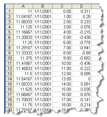
The Tidal Analysis and Prediction (TAP) software can perform tidal harmonic analysis and predictions of water levels and currents. The file format for tidal predictions contains 6 header lines with information on the file name, analysis length, tidal constituents used, goodness of fit parameters and vertical datums. The first column of data is the Julian day in Local Standard Time and the following three columns contain the observed, predicted and residual time series of water levels. Below is an example of the file format of a TAP’s Tidal Prediction File
- NAPL20010111.txt -- 20 day analysis --
- Start Date/Time(LST): 11-Jan-2001 00:00:00 11
- Tides: O1 K1 MNS2 N2 M2 S2 MK3 MN4 M4 S4 2MS6
- RMS= 0.099 %R_var= 86.42
- Mean water level: -0.1851 meters
- JDay(LST) Observed Predicted Residual
- 11.000000 0.3110 0.3257 -0.0147
- 11.041667 0.2800 0.3162 -0.0362
- 11.083333 0.2330 0.2213 0.0117
- 11.125000 0.0760 0.0387 0.0373
- 11.166667 -0.2150 -0.2053 -0.0097
Getting Started
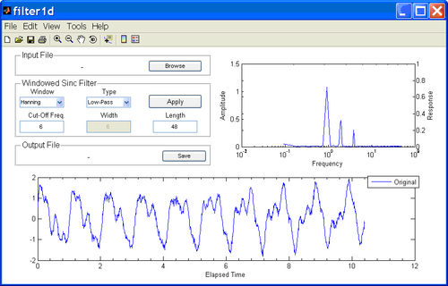
Filter1D is launched from the SMS 10.1+ interface. If the user has not already installed Filter1D during the SMS installation process, the user may install Filter1D by running the Matlab Component Runtime MCRinstaller.exe located in the main SMS directory. This file contains the Matlab libraries needed to run the program. There are two options to open the Filter1D utility. The first is by clicking on the menu Data | Analysis | 1D Filter. The Filter1D interface will appear with an idealized time series as shown in Figure 1. The time series consists of three tidal harmonic constituents M2 (1.9324 cpd), O1 (0.9295 cpd), and M4 (3.8647 cpd) plus additional white noise. The upper right plot shows the computed amplitude spectra as a function of frequency (cpd). Because the white noise energy is distributed in a wide range of frequencies, it does not appear to be significant in the amplitude spectra. However, from the time series plot, it is clear the quality of the signal is significantly reduced by the presence of noise.
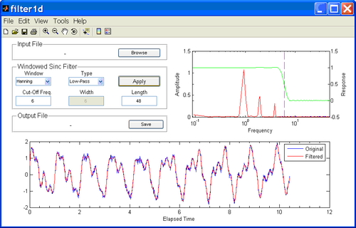
To filter the time series, simply click on the button labeled Apply. The resulting window is shown in Figure 2. In the menu which reads Windowed Sinc Filter, Window indicates the window used with the sinc function in the filter and Type indicates the type of filter and is either low-pass, high-pass and band-pass. Cut-Off Freq. indicates the cut-off frequency in the cases for low-pass and high-pass filters and the central frequency for Band-Pass filter. Length indicates the length of the filter or the number of weights used so that n = 2*Length+1 is the number of weights in the filter. The filtered time series will automatically be displayed in red in the lower plot. The amplitude spectrum plot will show an additional red line which corresponds to the calculated amplitude spectra of the filtered time series and allows the user to see how much energy has been removed from the time series in the frequency domain. Overlaid on the amplitude spectra plot is the filter response curve. The cut-off frequency is shown as a vertical line in the sample plot.
Although the original and filtered amplitude spectra are quite similar the reduction in noise is evident in the time series plot. It is recommended that the experiment with the many functions and options available using at this stage. For example, the data cursor
located in the menu bar may be used to click on any point of the time series or amplitude spectra plots to obtain the x- and y-values. The zoom in, zoom out
, and panning. tools are useful for view specific portions of long time series and inspecting the data for outliers. The markers (points) for the input and filtered time series can be displayed by selecting the option Line Markers under the View menu. It is recommended that the user change the filter settings inside the box labels "Windowed Sinc Filter" to get a good "feeling" for how the filter works.
Example Application
As an example, a water level time series measured by an Acoustic Doppler Profiler or ADP at Blind Pass, FL is analyzed and prepared for use in the Coastal Modeling System circulation model CMS-Flow. The user may obtain the input time series file Blind_Pass.tsd from the SMS wiki website <<< place link here>>>.
Loading Data and Initial Inspection
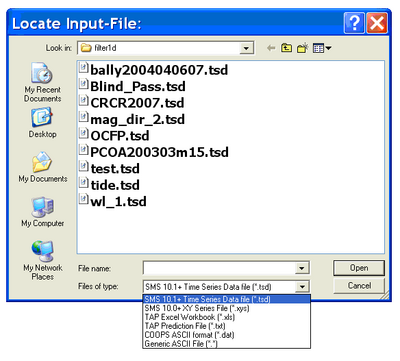
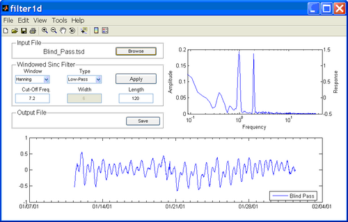
To load the data file Blind_Pass.tsd, click on the button labeled Browse and a window will appear as in Figure 3. Go to the folder where the input file is located, select the file and click on Open or simply double-click on the file.
After clicking OK, a dialog window will appear indicating that variables time steps have been identified. Since the filtering algorithm requires data spaced at regular intervals, the data must be interpolated to eliminate small data gaps, time shifts or changing in the sampling interval. The user will also be prompted to input the maximum interval for interpolation. The data is subsequently cropped to the first interval exceeding this value. By cropping the data in this way, the interpolation of large gaps is avoided which can introduce errors in the filter algorithm.
Once, the data is loaded, the Filter1D window should view as in Figure 4. The amplitude spectrum shows two distinct peaks at approximately 0.98 cpd and 1.93 cpd which correspond to the K1 and M2 tidal constituents respectively.
Initial Outlier Detection
Even before performing any filtering, the user may want to identify outliers and remove them from the time series. This is done by using maximum absolute value of the time series second derivative Points which exceed a user specified threshold are designated as possible outliers are highlighted with cyan colored squares. To identify possible outliers, click on Tools | Find Outliers. A window dialog will appear promting the user the input a threshold value. If the OK button is pressed, the points which exceed the threshold are highlighted but not deleted. In order to delete the points, the user must manually delete individual points by using the Delete Points tool under the Edit menu. To delete points, left-click on a point and a green circle will appear on the data point closest to the point clicked. An additional left-click on the point will remove it and linearly re-interpolate it. The default threshold is equal to four times the standard deviation of the maximum absolute second derivative for the whole time series.
Filtering
After clicking on the Apply button, the filtered time series and amplitude spectra will be displayed in red color. It is important to check that the cut-off frequency is adequate and that energy is not being removed at frequencies near the range of interest, in this, astronomical tides. The highest frequency of interest in case is the M4 tides (3.867 cpd). Therefore, a cut-off frequency of 5 cpd should be adequate. The best way of checking that the frequencies of interest are not being modified is by examining the amplitude spectra and filter response curve. It is also recommended to closely examine the time series by panning through sections of it after trying different cut-off frequencies and filter lengths to make sure that the user implements the optimal filter settings. In general, the closer the cut-off frequency is the frequencies of interest the sharper the response function must be and therefore the larger number of filter coefficients required. The disadvantage of using a larger number of filter coefficients is that the, the computation increases but mainly that the filter may have problems with start and ending of the time series. Filter1D automatically sets limits to the length of the filter.
Outlier Detection
Resampling and Interpolation
Calculator
Outliers are highlighted by This is done by checking the maximum absolute value of the second derivative of the data. Filter1D
This document shows an example of how to use the tool and uses real surface elevation data collected for Blind Pass, FL using and ADCP.
When Filter1D is started the following window will show on the screen. To load a data set, click on Browse in the Input File menu. TAP-Filt accepts ASCII input files with data arranged in columns. The value under Header Lines indicates how many lines to skip at the beginning of the input file. The value under Column indicates the column in which the input time-series is contained within the input file. Finally, the value under dt is the sampling period of the input data.
Set header lines to zero, column 3, dt to 0.3333.
In the menu which reads Windowed Sinc Filter, Window indicates the window used with the sinc function in the filter and Type indicates the type of filter and is either low-pass, high-pass and band-pass. Cut-Off Freq. indicates the cut-off frequency in the cases for low-pass and high-pass filters and the central frequency for Band-Pass filter. Length indicates the length of the filter or the number of weights used so that n = 2*Length+1 is the number of weights in the filter. Set the window to Lanczos, the cut-off frequency to 0.2 cycles/hr and the and the length equal to 30. Now load the file BlindPass_WL-MSL_Raw.dat using the Browse button in the Input File menu.
Additional Information
Questions about this CHETN can be addressed Alex Sánchez at (601-634-2027), FAX (601-634-3433), or e-mail: [mailto: Alejandro.Sanchez@usace.army.mil Alejandro.Sanchez@usace.army.mil]. This Technical Note should be referenced as follows:
References
Bloomfield, P. (1976). "Fourier Analysis of Time Series: An Introduction." John Wiley & Sons, New York, 258 pp.
Boon, J. D. (2004). "Secrets of the Tide: Tide and Tidal Current analysis and Predictions, Storm surges and Sea Level Trends." Horwood Publishing, Chichester, U.K. 212 pp.
Cartwright, D. E. (2000). "Tides: A scientific history." Cambridge University Press, 292 pp.
Doodson, A. T., and Warburg, H. D. (1944). "Admiralty Manual of Tides." Admiralty Charts and Publications, London, England, 270 pp.
Munk, W. H. and Cartwright, D. E. (1966). "Tidal Spectroscopy and Prediction." Phil. Trans. Royal Society of London. Series A, Mathematical and Physical Sciences, Vol. 259, No. 1105, pp. 533-581.
Pugh, D. T. (2004). "Changing Sea Levels: Effects of Tides, Weather and Climate." Cambridge University Press, 265 pp.
Schureman, P. (1958). "Manual of Harmonic Analysis and Prediction of Tides." U.S. Dept of Commerce, Coast and Geodetic Survey. Special Publication No. 98, Washington, D.C., 317 pp.
Appendix A
The sinc function is calculated as
| (1) |
where is the cut-off frequency. The following windows are available in Filter1D:
- Hanning
| Failed to parse (SVG with PNG fallback (MathML can be enabled via browser plugin): Invalid response ("Math extension cannot connect to Restbase.") from server "https://en.wikipedia.org/api/rest_v1/":): {\displaystyle w(i)=1/2(1-\cos{2\pii/N}) } | (2) |
The convolution of Equation (1) with a digital signal results
The filtered time series
is obtained by convolving the input time series
with the the filter weights
|
|
(1)
|
