LSTF: Difference between revisions
| Line 80: | Line 80: | ||
|} | |} | ||
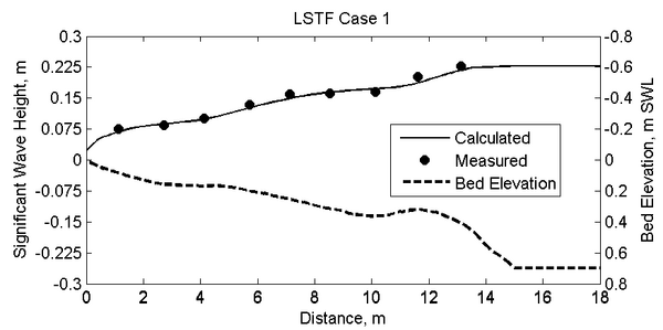
[[Image:LSTF_C1_WavePro.png|thumb| | [[Image:LSTF_C1_WavePro.png|thumb|left|600px|Figure 1. Computed and measured significant wave heights for LSTF Case 1.]] | ||
[[Image:LSTF_C1_CurrentPro.png|thumb| | [[Image:LSTF_C1_CurrentPro.png|thumb|left|600px|Figure 2. Computed and measured longshore currents for LSTF Case 1.]] | ||
[[Image:LSTF_C1_ElevPro.png|thumb| | [[Image:LSTF_C1_ElevPro.png|thumb|left|600px|Figure 3. Computed and measured mean water levels for LSTF Case 1.]] | ||
<br style="clear:both" /> | <br style="clear:both" /> | ||
| Line 142: | Line 142: | ||
|align = "center"|38.93 | |align = "center"|38.93 | ||
|} | |} | ||
Figure 4. Computed and measured longshore sediment transport rates LSTF Case 1 using the Lund-CIRP formulas. | |||
[[Image:LSTF_C1_SedPro_Lund-CIRP.png|thumb|left|600px|Figure 4. Computed and measured longshore sediment transport rates LSTF Case 1 using the Lund-CIRP formulas.]] | |||
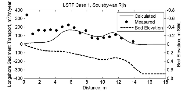
Figure 5. Computed and measured longshore sediment transport rates LSTF Case 1 using the Soulsby-van Rijn formulas. | |||
[[Image:LSTF_C1_SedPro_Soulsby-van_Rijn.png|thumb|left|600px|Figure 5. Computed and measured longshore sediment transport rates LSTF Case 1 using the Soulsby-van Rijn formulas.]] | |||
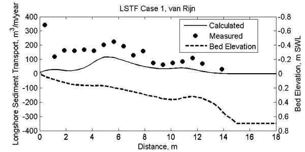
Figure 6. Computed and measured longshore sediment transport rates LSTF Case 1 using the van Rijn formulas. | |||
[[Image:LSTF_C1_SedPro_van_Rijn.png|thumb|left|600px|Figure 6. Computed and measured longshore sediment transport rates LSTF Case 1 using the van Rijn formulas.]] | |||
<br style="clear:both" /> | |||
==References== | ==References== | ||
Revision as of 22:24, 22 October 2010
Experimental Setup
The Large-Scale Sediment transport Facility (LSTF) at the Engineer Research and Development Center of U.S. Army Corps of Engineers (shown in Figure 1) is capable of simulate oblique (6.5º incident angle) regular and random waves and a uniform longshore current by adjusting a series of 20 pumps in the cross-shore direction therefore simulating an infinite beach. The test cases shown here represent natural beaches with uniform longshore currents (Cases 1-4). Each experiment was 160 minutes long. In Case 1, a longshore current was induced by oblique random waves and the pumps where adjusted to match the measured longshore current. Case 2 was ran with the same wave heights as Case 1, but the pumps were set to recirculate twice the measured longshore flux of Case 1. Because the model does not have a variable flux boundary condition, this is was not simulated. In Case 3, the wave generator was turned off, and only the pumps were run. For this reason, Case 3 was also not used to test the model.
Figure 1. LSTF configuration (Gravens and Wang 2007)
Model Setup
The computational domain was generated based on the interpolation of measured beach profiles from profile Y14 to Y34 (see Figure 1). A constant grid resolution of 0.2 and 0.4 m where was used in the cross-shore and longshore directions respectively. A TMA spectrum was assumed at the offshore boundary with the parameter values γ = 3.3, and n = 100. The offshore water level during the experiment is not equal to the Still Water Level (SWL) because of the wave setup. The offshore water level was approximated for each experiment based on the most offshore water level gauge.
Table 2. CMS-Flow Settings
| Setting | Value |
| Solver | Implicit |
| Time step | 60 sec |
| Wetting and drying depth | 0.001 m |
| Simulation duration | 3 hr |
| Ramp duration | 3 hr |
| Clock time | 2.08 min |
Table 3. CMS-Wave settings
| Setting | Value |
| Wave breaking | Jansen and Battjes |
| Diffraction coefficient | 3 |
| Bottom friction | Off |
| Steering interval | 0.25 hr |
Results
Measured wave heights, water levels, and depth-averaged current velocities were compared to the center line profile measurements in Figures 1 through 6.
Table 4. Offshore significant wave height Hmo, peak wave period Tp,, incident wave period Θo, water level η0 for the LSTF test cases.
| Hmo, m | Tp, s | Θo, deg | η0, m | |
| Case 1 | 0.228 | 1.465 | 6.5 | -0.001 |
| Case 2 | 0.228 | 1.465 | 6.5 | |
| Case 4 | 0.222 | 1.465 | 6.5 |
Table 5. Goodness of fit statistics for LSTF Case 1 for waves, water levels and longshore currents
| Hs, m | Eta, m | V, m/s | |
| RMSE | 0.0083 | 0.0012 | 0.0393 |
| RMAE | 0.0201 | 0.0261 | 0.0393 |
| R2 | 0.982 | 0.934 | 0.665 |
| Bias | 0.005 | 0.0001 | -0.017, |
Table 6. Goodness of fit statistics for LSTF Case 1 for waves, water levels and longshore currents
| Lund-CIRP Qt, m3/m/year |
van Rijn Qt, m3/m/year |
Soulsby-van Rijn Qt, m3/m/year | |
| RMSE | 57.21 | 87.82 | 72.90 |
| RMAE | 0.118 | 0.357 | 0.1738 |
| R2 | 0.20 | 0.57 | 0.10 |
| Bias | 26.43 | 79.92 | 38.93 |
References
- Gravens, M.B., Wang, P. (2007). "Data report: laboratory testing of longshore sand transport by waves and currents; morphology change behind headland structures". Technical Report, ERDC/CHL TR-07-8, Coastal and Hydraulics Laboratory, US Army Engineer Research and Development Center, Vicksburg, MS.


