Long wave propagation: Difference between revisions
No edit summary |
|||
| (6 intermediate revisions by the same user not shown) | |||
| Line 1: | Line 1: | ||
= | = Problem = | ||
Lynch and Gray (1978) presented the analytical solution for depth-averaged long-wave propagation in am annular domain. Here the case tested with a linearly sloping bed, and without bottom friction, Coriolis, or horizontal mixing. The offshore boundary consists of an single tidal constituent. Table 1 summarizes the important model settings used for this test. | |||
Table 1. General Settings for | '''Table 1. General Settings for quarter annulus test''' | ||
{|border="1" | {|border="1" | ||
|'''Parameter''' ||'''Value''' | |'''Parameter''' ||'''Value''' | ||
|- | |- | ||
|Deepwater | |Deepwater tidal amplitude|| 0.3048 m | ||
|- | |- | ||
|Tidal | |Tidal period || 12.42 hrs (M2) | ||
|- | |||
|Inner radius || 60.96 km | |||
|- | |||
|Outer radius || 152.4 km | |||
|- | |||
|Depth at inner radius || 10.02 m | |||
|- | |||
|Depth at outher || 25.05 m | |||
|- | |- | ||
|Bottom friction || None | |Bottom friction || None | ||
|- | |- | ||
|Horizontal eddy viscosity || | |Horizontal eddy viscosity || 0.0 | ||
|- | |||
|Corilis || 0.0 | |||
|} | |} | ||
= Model Setup = | = Model Setup = | ||
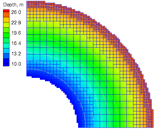
[[Image:QA_Depth_8km.png|thumb|right|600px| Figure 1. Quarter Annulus]] | |||
The computational domain (Figure 1) consists of a three-level telescoping Cartesian grid with a grid resolution of 4, 2, and 1 km for each level. Higher resolution is specified near the inner and outer boundaries in order to reduce errors associated with the representation of the curved boundaries with squares. The computational grid is shown in Figure 1. The grid has 1,160 active ocean cells. The important model settings are shown in Table 2. | |||
Table 2. General | '''Table 2. General settings for the quarter annulus test''' | ||
{|border="1" | {|border="1" | ||
|'''Parameter''' ||'''Value''' | |'''Parameter''' ||'''Value''' | ||
|- | |- | ||
|Time step|| 600 sec (10 min) | | Solution scheme || Implicit | ||
|- | |||
|Time step || 600 sec (10 min) | |||
|- | |||
|Simulation duration || 120 hrs | |||
|- | |- | ||
|Ramp period || 24 hrs | |Ramp period || 24 hrs | ||
|- | |- | ||
| | |Advection terms || Off | ||
|- | |- | ||
| | |Mixing terms || Off | ||
|- | |- | ||
| | |Wall friction || Off | ||
|- | |- | ||
| | |Coriolis || Off | ||
|} | |} | ||
<br style="clear:both" /> | |||
= Results = | = Results = | ||
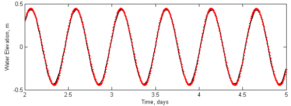
[[Image:QA_Water_Level_8km.png|thumb|right|600px| Figure 2. Comparison of analytical (solid black) and calculated (red dots) water surface elevation at the center of the inner radius. ]] | |||
Figure 2 shows a time series of water levels at the inner edge of the model domain. The goodness of fit statistics are listed in Table 3. The model accurately predicts the wave phase but slightly overestimates the amplitude by approximately 0.01 m. No significant numerical dissipation is observed or numerical instabilities. The simulation takes about 52 seconds on a PC and a single processor. | |||
Table 3. Goodness of fit statistics for the water elevation | '''Table 3. Goodness of fit statistics for the water elevation''' | ||
{|border="1" | {|border="1" | ||
|'''Statistic''' ||'''Value''' | |'''Statistic''' ||'''Value''' | ||
|- | |- | ||
| | |NRMSE || 3.3 % | ||
|- | |- | ||
| | |NRMAE || 2.7 % | ||
|- | |- | ||
|R^2 || 0.999 | |R^2 || 0.999 | ||
|- | |- | ||
|Bias || 0. | |Bias || 0.002 m | ||
|} | |} | ||
<br style="clear:both" /> | |||
= References = | = References = | ||
* Lynch, D.R., and Gray, W.G. (1978). "Analytical solutions for computer flow model testing," J. Hydraulics Division, 104, 1409-28. | * Lynch, D.R., and Gray, W.G. (1978). "Analytical solutions for computer flow model testing," J. Hydraulics Division, 104, 1409-28. | ||
Latest revision as of 23:15, 1 June 2011
Problem
Lynch and Gray (1978) presented the analytical solution for depth-averaged long-wave propagation in am annular domain. Here the case tested with a linearly sloping bed, and without bottom friction, Coriolis, or horizontal mixing. The offshore boundary consists of an single tidal constituent. Table 1 summarizes the important model settings used for this test.
Table 1. General Settings for quarter annulus test
| Parameter | Value |
| Deepwater tidal amplitude | 0.3048 m |
| Tidal period | 12.42 hrs (M2) |
| Inner radius | 60.96 km |
| Outer radius | 152.4 km |
| Depth at inner radius | 10.02 m |
| Depth at outher | 25.05 m |
| Bottom friction | None |
| Horizontal eddy viscosity | 0.0 |
| Corilis | 0.0 |
Model Setup

The computational domain (Figure 1) consists of a three-level telescoping Cartesian grid with a grid resolution of 4, 2, and 1 km for each level. Higher resolution is specified near the inner and outer boundaries in order to reduce errors associated with the representation of the curved boundaries with squares. The computational grid is shown in Figure 1. The grid has 1,160 active ocean cells. The important model settings are shown in Table 2.
Table 2. General settings for the quarter annulus test
| Parameter | Value |
| Solution scheme | Implicit |
| Time step | 600 sec (10 min) |
| Simulation duration | 120 hrs |
| Ramp period | 24 hrs |
| Advection terms | Off |
| Mixing terms | Off |
| Wall friction | Off |
| Coriolis | Off |
Results

Figure 2 shows a time series of water levels at the inner edge of the model domain. The goodness of fit statistics are listed in Table 3. The model accurately predicts the wave phase but slightly overestimates the amplitude by approximately 0.01 m. No significant numerical dissipation is observed or numerical instabilities. The simulation takes about 52 seconds on a PC and a single processor.
Table 3. Goodness of fit statistics for the water elevation
| Statistic | Value |
| NRMSE | 3.3 % |
| NRMAE | 2.7 % |
| R^2 | 0.999 |
| Bias | 0.002 m |
References
- Lynch, D.R., and Gray, W.G. (1978). "Analytical solutions for computer flow model testing," J. Hydraulics Division, 104, 1409-28.