CR-07-1:Chapter4: Difference between revisions
| (97 intermediate revisions by the same user not shown) | |||
| Line 1: | Line 1: | ||
__TOC__ | __TOC__ | ||
<big>NOTE: Tables 34 through 40 need to be entered</big> | |||
==Suspended load== | ==Suspended load== | ||
===Introduction=== | ===Introduction=== | ||
The earliest transport rate formulas are mainly based on the concept that the sediment transport rate for steady uniform flow can be related to the bottom shear stress (Meyer-Peter and Müller 1948; Einstein 1950; Engelund and Hansen 1972) assuming that bed-load transport prevails. However, if the shear stress is sufficiently large, the particles can be lifted, put in suspension, and transported in large quantities by the current. Thus, suspended load often prevails for fine sediments (''d''<sub>50</sub> < 0.5 mm). The traditional approach for calculating the unsteady depth-averaged volumetric suspended load transport ''q''<sub>''ss''</sub> is to determine the vertical distribution of suspended sediment concentration (''c'') and velocity (''u''), after which the product between these two quantities is integrated through the vertical from the edge of the bed-load layer (''z'' = ''z''<sub>''a''</sub>) to the water surface (''z'' = ''h'') (Van Rijn 1993), yielding: | The earliest transport rate formulas are mainly based on the concept that the sediment transport rate for steady uniform flow can be related to the bottom shear stress (Meyer-Peter and Müller 1948; Einstein 1950; Engelund and Hansen 1972) assuming that bed-load transport prevails. However, if the shear stress is sufficiently large, the particles can be lifted, put in suspension, and transported in large quantities by the current. Thus, suspended load often prevails for fine sediments (''d''<sub>50</sub> < 0.5 mm). The traditional approach for calculating the unsteady depth-averaged volumetric suspended load transport ''q''<sub>''ss''</sub> is to determine the vertical distribution of suspended sediment concentration (''c'') and velocity (''u''), after which the product between these two quantities is integrated through the vertical from the edge of the bed-load layer (''z'' = ''z''<sub>''a''</sub>) to the water surface (''z'' = ''h'') (Van Rijn 1993), yielding: | ||
{{Equation|<math>{{q}_{ss}}\left( t \right)=\int_{{{z}_{a}}}^{h}{u\left( z,t \right)c\left( z,t \right)dz}</math>|111}} | {{Equation|<math> | ||
{{q}_{ss}}\left( t \right)=\int_{{{z}_{a}}}^{h}{u\left( z,t \right)c\left( z,t \right)dz} | |||
</math>|111}} | |||
where ''q''<sub>''ss''</sub>(''t'') is the depth-averaged instantaneous suspended load per unit width, ''u''(''z'',''t'') and ''c''(''z'',''t'') are, respectively, the horizontal velocity and the volume sediment concentration at the height ''z'', ''z''<sub>''a''</sub> is the level at the top of the bed-load layer, and ''h''(''t'') is the instantaneous water depth. A steady situation is typically assumed to simplify the problem, so time-averaged values <math>u\left( z \right)=\overline{u\left( z,t \right)}</math> and | where ''q''<sub>''ss''</sub>(''t'') is the depth-averaged instantaneous suspended load per unit width, ''u''(''z'',''t'') and ''c''(''z'',''t'') are, respectively, the horizontal velocity and the volume sediment concentration at the height ''z'', ''z''<sub>''a''</sub> is the level at the top of the bed-load layer, and ''h''(''t'') is the instantaneous water depth. A steady situation is typically assumed to simplify the problem, so time-averaged values <math>u\left( z \right)=\overline{u\left( z,t \right)}</math> and <math>c\left( z \right)=\overline{c\left( z,t \right)}</math> | ||
<math>c\left( z \right)=\overline{c\left( z,t \right)}</math> | |||
are substituted (Figure 39): | are substituted (Figure 39): | ||
{{Equation|<math> | {{Equation|<math> | ||
q_{ss}=\int_{z_a}^{h}{c\left( z \right)u\left( z \right)dz} | |||
</math>|112}} | |||
Therefore, an accurate estimation of the total suspended load requires accurate prediction of the mean current velocity and concentration profiles. | Therefore, an accurate estimation of the total suspended load requires accurate prediction of the mean current velocity and concentration profiles. | ||
| Line 23: | Line 30: | ||
To describe suspended load above the wave boundary layer, some refined mathematical approaches were proposed during the last decades with sophisticated turbulence closure models (Fredsøe et al. 1985; Davies 1990; Davies et al. 1997). However, the development of practical sediment transport models still has a strong empirical character and relies heavily on physical insight combined with quantitative data obtained through laboratory and field experiments. | To describe suspended load above the wave boundary layer, some refined mathematical approaches were proposed during the last decades with sophisticated turbulence closure models (Fredsøe et al. 1985; Davies 1990; Davies et al. 1997). However, the development of practical sediment transport models still has a strong empirical character and relies heavily on physical insight combined with quantitative data obtained through laboratory and field experiments. | ||
An essential part of morphodynamic computations for flow conditions involving suspended sediment transport is the use of a reference concentration as a bed boundary condition. Van Rijn (1984b) proposed that the reference concentration should be a function of the bed-load transport. Furthermore, the main controlling parameters for the suspended load are the settling velocity of the sediment ''W''<sub>''s''</sub>, and more specifically, the vertical sediment diffusion coefficient | An essential part of morphodynamic computations for flow conditions involving suspended sediment transport is the use of a reference concentration as a bed boundary condition. Van Rijn (1984b) proposed that the reference concentration should be a function of the bed-load transport. Furthermore, the main controlling parameters for the suspended load are the settling velocity of the sediment ''W''<sub>''s''</sub>, and more specifically, the vertical sediment diffusion coefficient <math>\varphi_v</math>. The latter is examined here and compared to the Van Rijn (1984b) results. | ||
In the nearshore, for mild wave conditions, the bed is covered by ripples. These bed forms strongly affect the sediment transport by enhancing the suspended load, but also by modifying the direction of the sediment transport. Assuming | In the nearshore, for mild wave conditions, the bed is covered by ripples. These bed forms strongly affect the sediment transport by enhancing the suspended load, but also by modifying the direction of the sediment transport. Assuming <math>u\left( z,t \right)=\overline{u\left( z,t \right)}+\overline{u}\left( z,t \right)=u\left( z \right)+\overline{u}\left( z,t \right)</math> and <math>c\left( z,t \right)=\overline{c\left( z,t \right)}+\overline{c}\left( z,t \right)=c\left( z \right)+\overline{c}\left( z,t \right)</math>, where <math>\overline{u}\left( z,t \right)</math> and | ||
<math>\overline{c}\left( z,t \right)</math> are the oscillatory components, the net suspended sediment transport is obtained by averaging Equation 111: | |||
<math> | {{Equation|<math> | ||
q_{ss}=<\int_{{{z}_{a}}}^{h\left( t \right)}{\left[ u\left( z \right)c\left( z \right)+\overline{u}\left( z,t \right)\overline{c}\left( z,t \right) \right]}dz> | |||
</math>|113}} | |||
{{Equation|<big><math> =q_{ss,c} + q_{ss,w} </math></big>|114}} | |||
{{Equation|< | |||
The first term on the right side (Equation 114) corresponds to the current-related suspended load, and the second term corresponds to the wave-related suspended load. The wave-related suspended load includes the quasi-steady suspended load due to asymmetric waves (assuming no phase lag exist between the wave velocity and the sediment concentration) and the unsteady effects due to a possible phase lag between the instantaneous velocity and concentration. Many experimental studies and most predictive models do not take into account the wave-related suspended load, although it appears to be significant for cross-shore sediment transport. | The first term on the right side (Equation 114) corresponds to the current-related suspended load, and the second term corresponds to the wave-related suspended load. The wave-related suspended load includes the quasi-steady suspended load due to asymmetric waves (assuming no phase lag exist between the wave velocity and the sediment concentration) and the unsteady effects due to a possible phase lag between the instantaneous velocity and concentration. Many experimental studies and most predictive models do not take into account the wave-related suspended load, although it appears to be significant for cross-shore sediment transport. | ||
| Line 52: | Line 46: | ||
===Equilibrium profile for suspended sediment=== | ===Equilibrium profile for suspended sediment=== | ||
'''Mass conservation equation''' | |||
An equilibrium can exist between the settling velocity and the hydrodynamic forcing (Figure 40). The equation for the sediment concentration is derived from the mass conservation equation employed to compute changes in bottom topography: | An equilibrium can exist between the settling velocity and the hydrodynamic forcing (Figure 40). The equation for the sediment concentration is derived from the mass conservation equation employed to compute changes in bottom topography: | ||
{{Equation|<math>\frac{\partial c}{\partial t}+\text{div}\vec{F}=0</math>|115}} | {{Equation|<math>\frac{\partial c}{\partial t}+\text{div}\vec{F}=0 </math>|115}} | ||
with | with | ||
{{Equation|<math>\vec{F}={{\vec{F}}_{a}}+{{\vec{F}}_{s}}+{{\vec{F}}_{d}}</math>|116}} | {{Equation|<math>\vec{F}={{\vec{F}}_{a}}+{{\vec{F}}_{s}}+{{\vec{F}}_{d}} </math>|116}} | ||
where ''c'' is the sediment volume concentration (dimensionless), and ''F'' is the total sediment flux (consisting of contributions from advection, settling, and diffusion): | where ''c'' is the sediment volume concentration (dimensionless), and ''F'' is the total sediment flux (consisting of contributions from advection, settling, and diffusion): | ||
{{Equation|<math>\begin{align} | {{Equation|<math> | ||
& {{{\vec{F}}}_{a}}=c\ \vec{u}+c\ w\ {{{\vec{e}}}_{z}} \\ | \begin{align} | ||
& {{{\vec{F}}}_{s}}=-c\ {{W}_{s}}\ {{{\vec{e}}}_{z}} \\ | & {{{\vec{F}}}_{a}}=c\ \vec{u}+c\ w\ {{{\vec{e}}}_{z}} \\ | ||
& {{{\vec{F}}}_{d}}=-{{\varepsilon }_{h}}\ \overrightarrow{\text{gra}{{\text{d}}_{\text{h}}}}\left( c \right)-{{\varepsilon }_{\nu }}\frac{\partial c}{\partial z}{{{\vec{e}}}_{z}} \\ | & {{{\vec{F}}}_{s}}=-c\ {{W}_{s}}\ {{{\vec{e}}}_{z}} \\ | ||
\end{align}</math>|117}} | & {{{\vec{F}}}_{d}}=-{{\varepsilon }_{h}}\ \overrightarrow{\text{gra}{{\text{d}}_{\text{h}}}}\left( c \right)-{{\varepsilon }_{\nu }}\frac{\partial c}{\partial z}{{{\vec{e}}}_{z}} \\ | ||
\end{align} | |||
</math>|117}} | |||
with <math>\vec{u}</math> the horizontal velocity vector, ''w'' the vertical velocity, <math>{{\vec{e}}_{z}}</math> the unit vector in the vertical, | with <math>\vec{u}</math> the horizontal velocity vector, ''w'' the vertical velocity, <math>{{\vec{e}}_{z}}</math> the unit vector in the vertical, <math>\overrightarrow{\text{gra}{{\text{d}}_{\text{h}}}}=\partial /\partial x+\partial /\partial y</math> the horizontal gradient, and <math>\varepsilon_v</math> and <math>\varepsilon_h</math> the vertical and horizontal eddy diffusivity, respectively. | ||
<math>\overrightarrow{\text{gra}{{\text{d}}_{\text{h}}}}=\partial /\partial x+\partial /\partial y</math> | |||
the horizontal gradient, and | |||
The bottom boundary condition yields the following relationship: | The bottom boundary condition yields the following relationship: | ||
{{Equation|<math>-\left( {{{\vec{F}}}_{s}}+{{{\vec{F}}}_{d}} \right)\ \vec{n}=S</math>|118}} | {{Equation|<math> | ||
-\left( {{{\vec{F}}}_{s}}+{{{\vec{F}}}_{d}} \right)\ \vec{n}=S | |||
</math>|118}} | |||
where <math>\vec{n}</math> is the unit vector perpendicular to the bottom, and ''S'' the erosion-deposition flux due to suspended load. | where <math>\vec{n}</math> is the unit vector perpendicular to the bottom, and ''S'' the erosion-deposition flux due to suspended load. | ||
[[Image:CR-07-1_Chapter4_02.jpg|500px|none]] | [[Image:CR-07-1_Chapter4_02.jpg|500px|none]] | ||
| Line 83: | Line 79: | ||
'''Figure 40. Concentration profile for steady conditions.''' | '''Figure 40. Concentration profile for steady conditions.''' | ||
Several different expressions have been derived for the concentration profile, but most of them rely on the steady-state vertical diffusion equation (Figure 40). Under steady conditions (<math>\partial c/\partial t=0</math>, <math>\text{div}{{\vec{F}}_{a}}=0</math>, <math>\overrightarrow{\text{gra}{{\text{d}}_{\text{h}}}}\left( c \right)=0\ \text{and}\ S=0</math>), Equation 115 may be simplified to: | Several different expressions have been derived for the concentration profile, but most of them rely on the steady-state vertical diffusion equation (Figure 40). Under steady conditions (<math>\partial c/\partial t=0</math>, <math>\text{div}{{\vec{F}}_{a}}=0</math>, <math>\overrightarrow{\text{gra}{{\text{d}}_{\text{h}}}}\left( c \right)=0\ \text{and}\ S=0</math>), Equation 115 may be simplified to: | ||
{{Equation|<math>\frac{\partial c\left( z \right)}{\partial z}+\frac{{{W}_{s}}}{{{\varepsilon }_{v}}}c\left( z \right)=0</math>|119}} | {{Equation|<math> | ||
\frac{\partial c\left( z \right)}{\partial z}+\frac{{{W}_{s}}}{{{\varepsilon }_{v}}}c\left( z \right)=0 | |||
</math>|119}} | |||
Depending on the expression selected for | Depending on the expression selected for <math>\varepsilon_v</math> analytical solutions to Equation 119 of different type may be found. Thus, if <math>c\left( z={{z}_{a}} \right)={{c}_{a}}</math>, where ''z''<sub>''a''</sub> is the reference level (the maximum value of the computed roughness is often used): | ||
{{Equation|<math>c\left( z \right)={{c}_{a}}\exp \left( -\int_{{{z}_{a}}}^{z}{\frac{Ws}{{{\varepsilon }_{v}}}dz} \right)</math>|120}} | {{Equation|<math> | ||
c\left( z \right)={{c}_{a}}\exp \left( -\int_{{{z}_{a}}}^{z}{\frac{Ws}{{{\varepsilon }_{v}}}dz} \right) | |||
</math>|120}} | |||
'''Schmidt number''' | |||
An eddy viscosity coefficient is employed for determining the mixing, or diffusion coefficient. However, the mixing of sediment is not completely analogous to the mixing of water. The vertical eddy diffusivity of particles | An eddy viscosity coefficient is employed for determining the mixing, or diffusion coefficient. However, the mixing of sediment is not completely analogous to the mixing of water. The vertical eddy diffusivity of particles <math>\varepsilon_v</math> is then related to the vertical eddy viscosity V<sub>''v''</sub> through the Schmidt number s: | ||
{{Equation|<math>\sigma =\frac{{{\varepsilon }_{v}}}{{{\nu }_{v}}}</math>|121}} | {{Equation|<math>\sigma =\frac{{{\varepsilon }_{v}}}{{{\nu }_{v}}} </math>|121}} | ||
In principle, | In principle, s should be a constant, and s = 1. Three different processes were listed by Rose and Thorne (2001) to explain a deviation from unity: | ||
* The first process to explain a | * The first process to explain a s-values different from unity was proposed by Sumer and Deigaard (1981) and Van Rijn (1984b). They hypothesized that the centrifugal force in a fluid eddy causes sediment grains to be thrown outside of the eddy, which increases s. | ||
* Another reason presented by Fredsøe and Deigaard (1994, pp. 231-234) for | * Another reason presented by Fredsøe and Deigaard (1994, pp. 231-234) for s to deviate from unity might be sediment settling out of the surrounding water before the water loses its earlier composition by mixing. This effect is particularly significant for the high concentration of cohesive sediments. Lees (1981) showed that s displayed a decreasing trend with increasing suspended sediment concentration. | ||
* Rose and Thorne (2001) added that the estimation of | * Rose and Thorne (2001) added that the estimation of s may be affected by the settling velocity, which varies because of the presence of turbulence. | ||
Based on measurements by Coleman (1981), Van Rijn (1984b) suggested the following expression for | Based on measurements by Coleman (1981), Van Rijn (1984b) suggested the following expression for s, which was defined as the ratio between the maximum sediment diffusivity and the maximum fluid eddy viscosity (<math>\sigma ={{\varepsilon }_{v,\max }}/{{\nu }_{v,\max }}</math> with <math>{{\nu }_{v,\max }}=0.25\ \kappa {{u}_{*}}h</math> for a parabolic profile): | ||
{{Equation|<math>\sigma =1+2{{\left( \frac{ | {{Equation|<math> | ||
\sigma =1+2 { {\left( \frac{W_s}{u_*} \right)}^2}\text{ with }0.1<\frac{W_s}{u_*}<1 | |||
</math>|122}} | |||
'''Sediment diffusivity and concentration profiles''' | |||
The sediment diffusivity | The sediment diffusivity <math>\varepsilon_v</math> is a fundamental parameter for the estimation of the concentration profile, and it is a function of bottom roughness and shear stress, agitation (mainly due to waves), and settling velocity. Various distributions of the sediment mixing can be found in the literature, which typically produce either an exponential or a power-law sediment concentration profile. | ||
''Exponential profile''. If the sediment diffusivity | ''Exponential profile''. If the sediment diffusivity <math>\varepsilon_v</math> is constant (<math>\varepsilon_v \approx 10^-12 m^2</math>), an exponential profile is obtained for the mean concentration: | ||
{{Equation|<math>c\left( z \right)={{c}_{R}}\exp \left( -\frac{{{W}_{s}}}{{{\varepsilon }_{v}}}z \right)</math>|123}} | {{Equation|<math> | ||
c\left( z \right)={{c}_{R}}\exp \left( -\frac{{{W}_{s}}}{{{\varepsilon }_{v}}}z \right) | |||
</math>|123}} | |||
where ''c''<sub>''R''</sub> is the reference concentration. The ratio ''W''<sub>''s''</sub>/ | where ''c''<sub>''R''</sub> is the reference concentration. The ratio ''W''<sub>''s''</sub>/<math>\varepsilon_v</math> determines suspension conditions: | ||
if ''W''<sub>''s''</sub>/ | if ''W''<sub>''s''</sub>/<math>\varepsilon_v</math> > 4: weak suspension, | ||
if ''W''<sub>''s''</sub>/ | if ''W''<sub>''s''</sub>/<math>\varepsilon_v</math> < 0.5: strong suspension. | ||
The sediment diffusivity is often described as a function of the shear velocity and the water depth according to: | The sediment diffusivity is often described as a function of the shear velocity and the water depth according to: | ||
{{Equation|<math>{{\varepsilon }_{v,E}}={{\sigma }_{E}}\ \kappa \ {{u}_{*}}\ h</math>|124}} | {{Equation|<math>{{\varepsilon }_{v,E}}={{\sigma }_{E}}\ \kappa \ {{u}_{*}}\ h </math>|124}} | ||
where | where <math>\kappa</math> is Von Karman's constant (<math>\kappa</math> = 0.41), and s<sub>''E''</sub> a constant consistent with the Schmidt number s. | ||
''Power-law | ''Power-law profile''. In the coastal zone, <math>\varepsilon_v</math> is typically not expected to be constant over the depth, but a function of the agitation (mainly due to waves), bottom roughness, and settling velocity. For suspended sediment in a steady current, Rouse (1938) proposed a linear equation for the sediment diffusivity: | ||
{{Equation|<math>{{\varepsilon }_{v,P}}={{\sigma }_{P}}\ \kappa \ {{u}_{*}}\ z</math>|125}} | {{Equation|<math> | ||
{{\varepsilon }_{v,P}}={{\sigma }_{P}}\ \kappa \ {{u}_{*}}\ z | |||
</math>|125}} | |||
with | with s<sub>''P''</sub> being a constant consistent with the Schmidt number s that Rouse assumed equal to 1. This expression, nowadays widely used, gives the following expression for the concentration profile over depth: | ||
{{Equation|<math>c\left( z \right)={{c}_{a}}{{\left( \frac{z}{{{z}_{a}}} \right)}^{-{{W}_{s}}/{{\sigma }_{p}}\kappa {{u}_{*}}}}</math>|126}} | {{Equation|<math> | ||
c\left( z \right)={{c}_{a}}{ {\left( \frac{z}{{{z}_{a}}} \right)}^{-{{W}_{s}}/{{\sigma }_{p}}\kappa {{u}_{*}}}} | |||
</math>|126}} | |||
The parameter | The parameter <math>P_R = W_s/(\kappa {u}{*})</math> is commonly referred to as the Rouse parameter. It determines the shape of the suspended sediment profile, whereas the reference concentration ''c''<sub>''a''</sub> determines the magnitude of sediment in suspension at the reference level ''a'': | ||
* ''P''<sub>''R''</sub> > 5: near-bed suspension (''h''/10). | * ''P''<sub>''R''</sub> > 5: near-bed suspension (''h''/10). | ||
| Line 140: | Line 148: | ||
The Rouse expression may be extended to a parabolic equation for the sediment diffusivity: | The Rouse expression may be extended to a parabolic equation for the sediment diffusivity: | ||
{{Equation|<math>{{\varepsilon }_{v,B}}={{\sigma }_{B}}\ \kappa \ {{u}_{*}}\ z\left( 1-\frac{z}{h} \right)</math>|127}} | {{Equation|<math> | ||
{{\varepsilon }_{v,B}}={{\sigma }_{B}}\ \kappa \ {{u}_{*}}\ z\left( 1-\frac{z}{h} \right) | |||
</math>|127}} | |||
where | where s<sub>''B''</sub> is a constant consistent with the Schmidt number s. This expression implies the following solution for concentration profile over the depth: | ||
{{Equation|<math>c\left( z \right)={{c}_{a}}{{\left( \frac{z}{h-z}\frac{h-{{z}_{a}}}{{{z}_{a}}} \right)}^{-{{W}_{s}}/{{\sigma }_{B}}\kappa {{u}_{*}}}}</math>|128}} | {{Equation|<math> | ||
c\left( z \right)={{c}_{a}}{ {\left( \frac{z}{h-z}\frac{h-{{z}_{a}}}{{{z}_{a}}} \right)}^{-{{W}_{s}}/{{\sigma }_{B}}\kappa {{u}_{*}}}} | |||
</math>|128}} | |||
Because | Because <math>\varepsilon_v</math> varies over the depth, different values for s<sub>''E''</sub>, s<sub>''P''</sub>, and s<sub>''B''</sub> are obtained depending on the chosen profile. Figure 41 plots the three different analytic profiles (Equations 124, 125, and 127) with s<sub>''E''</sub> = 1/2s<sub>''P''</sub> = 1/6s<sub>''B''</sub> assuming that the constant value for the sediment diffusivity was obtained from an average over the depth for the linear profile and the parabolic profile. | ||
''Experimental estimation of sediment diffusivity profile''. If reliable point-concentration measurements are available, | ''Experimental estimation of sediment diffusivity profile''. If reliable point-concentration measurements are available, <math>\varepsilon_v</math> may be calculated from (Vanoni 1946): | ||
{{Equation|<math>{{\varepsilon }_{v}}=\frac{-{{W}_{s}}c}{dc/dz}</math>|129}} | {{Equation|<math>{{\varepsilon }_{v}}=\frac{-{{W}_{s}}c}{dc/dz}</math>|129}} | ||
| Line 158: | Line 170: | ||
[[Image:CR-07-1_Chapter4_03_16.png|500px|none]] | [[Image:CR-07-1_Chapter4_03_16.png|500px|none]] | ||
'''Figure 41. Three analytical relationships for vertical sediment diffusivity (Equations 124, 125, and 127) versus ''''''''z''''''''/''''''''h'' ''''''with | '''Figure 41. Three analytical relationships for vertical sediment diffusivity (Equations 124, 125, and 127) versus ''''''''z''''''''/''''''''h'' ''''''with s = s'''<sub>'''''E''</sub> ''''''= 1/2s'''<sub>'''''P''</sub> ''''''= 1/6s'''<sub>'''''B'''''</sub>'''.''' | ||
===Sediment diffusivity due to steady current=== | ===Sediment diffusivity due to steady current=== | ||
'''Experimental data''' | |||
To investigate the sediment diffusivity profile in steady conditions, available data sets covering a wide range in conditions were compiled and analyzed. Table 15 summarizes these data sets, where the types of flow motion and sediment properties are listed. For all these experiments, sand with a relative density ''s'' = 2.65 was used. Most of these data sets were found in the SEDMOC (Van Rijn et al. 2001) data compilation. | To investigate the sediment diffusivity profile in steady conditions, available data sets covering a wide range in conditions were compiled and analyzed. Table 15 summarizes these data sets, where the types of flow motion and sediment properties are listed. For all these experiments, sand with a relative density ''s'' = 2.65 was used. Most of these data sets were found in the SEDMOC (Van Rijn et al. 2001) data compilation. | ||
| Line 256: | Line 268: | ||
The experimental values obtained from each sediment concentration profile in the data sets are plotted (Figure 43) using Equation 129 and a point-by-point method yielding an estimate of the diffusivity according to: | The experimental values obtained from each sediment concentration profile in the data sets are plotted (Figure 43) using Equation 129 and a point-by-point method yielding an estimate of the diffusivity according to: | ||
{{Equation|<math>{{\varepsilon }_{c,i}}=\frac{-{{W}_{s}}c(i)}{\left\{ c\left( i+1 \right)-c\left( i-1 \right)/\left[ z\left( i+1 \right)-z\left( i-1 \right) \right] \right\}}</math>|130}} | {{Equation|<math> | ||
{{\varepsilon }_{c,i}}=\frac{-{{W}_{s}}c(i)}{\left\{ c\left( i+1 \right)-c\left( i-1 \right)/\left[ z\left( i+1 \right)-z\left( i-1 \right) \right] \right\}} | |||
</math>|130}} | |||
where ''i'' + 1 indicates consecutive experimental points along the z-axis for the concentration profile, and | where ''i'' + 1 indicates consecutive experimental points along the z-axis for the concentration profile, and <math>\varepsilon</math><sub>''c,i''</sub> is the estimated sediment diffusivity at level ''z'' = ''z''(''i''). Figure 43 confirms several results obtained previously. First, the sediment diffusivity is a linear function of the shear velocity ''u''<sub>''*c''</sub> and the water depth ''h''. Nevertheless, it appears that the mean values obtained for ''z'' <math>\approx</math> ''h''/2 (where <math>\varepsilon_c</math> is not function of ''z''), depends on other parameters. Based on analysis of the different data set, the mean value varies from 710<sup> 2</sup> m<sup>2</sup>/sec to 1 m<sup>2</sup>/sec. Moreover, <math>\varepsilon_c</math> appears to be an increasing function of ''z'' if <math>z/h\le 0.3</math>, a constant value for <math>0.3\le z/h\le 0.7</math>, and a decreasing function of ''z'' if <math>z/h\le 0.7</math>. Thus, referring to these results and the curves obtained in Figure 41, the best of the three analytic profiles previously discussed is the parabolic profile (Equation 127). Van Rijn(1984b) also proposed the following equations to compute the current-related sediment diffusivity: | ||
{{Equation| | {{Equation|<math> | ||
\begin{align} | |||
\varepsilon_c &=\kappa \sigma {{u}_{*}}\ z(1-z/h) &\text{if}\quad {z}<0.5 h \\ | |||
&=0.25\kappa \sigma {{u}_{*}}\ h &\text{if}\quad 0.5 h<z | |||
\end{align} | |||
</math>|131}} | |||
Van Rijn (1984b) assumed that the sediment diffusivity is constant in the upper part of the water column. However, from the experimental results, a decrease is clearly observed if <math>z/h\le 0.7</math>. Equation 131, which produces a complex equation for the concentration profile, does not appear to improve the results compared to the parabolic profile. | Van Rijn (1984b) assumed that the sediment diffusivity is constant in the upper part of the water column. However, from the experimental results, a decrease is clearly observed if <math>z/h\le 0.7</math>. Equation 131, which produces a complex equation for the concentration profile, does not appear to improve the results compared to the parabolic profile. | ||
| Line 266: | Line 285: | ||
Finally, for the data sets from Voogt et al. (1991) and Damgaard et al. (2003), measurements of the energy slope were not made, and the calculation of the shear velocity from the velocity profile shows significant scatter. Therefore, results obtained for these two data sets are not presented in Figure 43. | Finally, for the data sets from Voogt et al. (1991) and Damgaard et al. (2003), measurements of the energy slope were not made, and the calculation of the shear velocity from the velocity profile shows significant scatter. Therefore, results obtained for these two data sets are not presented in Figure 43. | ||
'''Shape of concentration profile''' | |||
Power-law and exponential concentration profiles were fitted to the measurements (Table 15). For a power-law profile, both linear and parabolic sediment diffusivity were examined. Some typical examples of the fit for these profiles are presented in Figure 44 for each of the data sets. Table 16 lists the percentage of sediment concentration values predicted within a range of 20 percent error of the measurements presented for the different data sets (symbolized by ''pred''<sub>20,''meas''</sub>, ''pred''<sub>20,''powL''</sub>, and ''pred''<sub>20,''pow''</sub> for the fit of the exponential-law and the "linear" and "parabolic" power-laws, respectively in Figure 45). These calculations were also performed for sediment concentration data closer to the bed (''z ''< ''h''/3) and in the upper layer (''z'' > ''h''/3), where the velocity is approximately constant. | Power-law and exponential concentration profiles were fitted to the measurements (Table 15). For a power-law profile, both linear and parabolic sediment diffusivity were examined. Some typical examples of the fit for these profiles are presented in Figure 44 for each of the data sets. Table 16 lists the percentage of sediment concentration values predicted within a range of 20 percent error of the measurements presented for the different data sets (symbolized by ''pred''<sub>20,''meas''</sub>, ''pred''<sub>20,''powL''</sub>, and ''pred''<sub>20,''pow''</sub> for the fit of the exponential-law and the "linear" and "parabolic" power-laws, respectively in Figure 45). These calculations were also performed for sediment concentration data closer to the bed (''z ''< ''h''/3) and in the upper layer (''z'' > ''h''/3), where the velocity is approximately constant. | ||
| Line 293: | Line 312: | ||
'''Figure 43. Vertical profile of sediment diffusivity obtained from Equation 129 using measured concentration profiles (each symbol corresponds to a particular profile).''' | '''Figure 43. Vertical profile of sediment diffusivity obtained from Equation 129 using measured concentration profiles (each symbol corresponds to a particular profile).''' | ||
'''Table 16. Percentage of predictions of sediment concentration within +/- 20 percent of measured values obtained using an exponential law or power law <br>(linear and parabolic profile) for | '''Table 16. Percentage of predictions of sediment concentration within +/- 20 percent of measured values obtained using an exponential law or power law <br>(linear and parabolic profile) for <math>\varepsilon_c</math> in fitting against data. ''' | ||
{|border="2" cellspacing="0" cellpadding="4" width="100%" align="center" | {|border="2" cellspacing="0" cellpadding="4" width="100%" align="center" | ||
| Line 444: | Line 463: | ||
It should also be noted that the parabolic power-law profile produces a concentration equal to zero at the level ''z'' = ''h'', although the two other laws allows a non-zero value. In breaking waves, the sediment diffusivity is clearly different from zero at ''z'' = ''h'', which means that the parabolic power-law profile may not be used in the presence of breaking waves. For an expression that is applicable for both current and waves, the exponential law seems to be the most appropriate. | It should also be noted that the parabolic power-law profile produces a concentration equal to zero at the level ''z'' = ''h'', although the two other laws allows a non-zero value. In breaking waves, the sediment diffusivity is clearly different from zero at ''z'' = ''h'', which means that the parabolic power-law profile may not be used in the presence of breaking waves. For an expression that is applicable for both current and waves, the exponential law seems to be the most appropriate. | ||
'''Estimation of Schmidt number''' | |||
Based on concentration profiles obtained from the compiled data set (Table 15), the fitted power-law and exponential profiles allow for an estimate of the Schmidt number. As discussed previously, the parabolic power-law profile for the sediment diffusivity | Based on concentration profiles obtained from the compiled data set (Table 15), the fitted power-law and exponential profiles allow for an estimate of the Schmidt number. As discussed previously, the parabolic power-law profile for the sediment diffusivity ?<sub>''c''</sub> produces the best qualitative agreement with the observed profiles. For that reason, a good correlation between s<sub>''B''</sub> and s is expected, and s<sub>''B''</sub> is calculated using Equation 128: | ||
{{Equation|<math>{{\sigma }_{B}}=\frac{-{{W}_{s}}}{{{\alpha }_{B}}\kappa {{u}_{*c}}}</math>|132}} | {{Equation|<math> | ||
{{\sigma }_{B}}=\frac{-{{W}_{s}}}{{{\alpha }_{B}}\kappa {{u}_{*c}}} | |||
</math>|132}} | |||
where | where a<sub>''B''</sub> is the observed slope of the power-law relationship obtained by fitting to the data (the s<sub>''P''</sub>-value is obtained in a similar manner). | ||
Some additional data were compiled (Table 17) from the studies by Rose and Thorne (2001), who also estimated | Some additional data were compiled (Table 17) from the studies by Rose and Thorne (2001), who also estimated s<sub>c</sub> assuming a Rouse concentration profile, and from Van Rijn (1984b), who used the Coleman (1970)data. | ||
Combining data sets listed in Table 15 and the data listed in Table 17, a similar expression as the one Van Rijn (1984b) proposed was found (Figure 46): | Combining data sets listed in Table 15 and the data listed in Table 17, a similar expression as the one Van Rijn (1984b) proposed was found (Figure 46): | ||
{{Equation|<math>{{\sigma }_{c}}\approx {{\sigma }_{B}}=0.6+6{{\left( \frac{{{W}_{s}}}{{{u}_{*c}}} \right)}^{2}}</math>|133}} | {{Equation|<math> | ||
{{\sigma }_{c}}\approx {{\sigma }_{B}}=0.6+6{ {\left( \frac{{{W}_{s}}}{{{u}_{*c}}} \right)}^{2}} | |||
</math>|133}} | |||
'''Table 17. Data summary for analysis on Schmidt number (''''''''d'''''<sub>'''''''''s'</sub><sub>'</sub> ''''''corresponds to median grain size in suspension). ''' | '''Table 17. Data summary for analysis on Schmidt number (''''''''d'''''<sub>'''''''''s'</sub><sub>'</sub> ''''''corresponds to median grain size in suspension). ''' | ||
| Line 501: | Line 524: | ||
|}<br clear="all"> | |}<br clear="all"> | ||
This equation produces a critical value for | This equation produces a critical value for $W_s/u_{*c} \approx 0.25$, yielding $\sigma | ||
_c = 1$. Up to this critical value, the centrifugal forces in the fluid eddies produce an increasing $\sigma_c$. Equation 133 presents improved results compared to previous predictive formulas, as shown in Table 18 and Figure 46. | |||
'''Table 18. Prediction of Schmidt number using parabolic profile <br>or an exponential profile for steady current. ''' | '''Table 18. Prediction of Schmidt number using parabolic profile <br>or an exponential profile for steady current. ''' | ||
| Line 507: | Line 531: | ||
{|border="2" cellspacing="0" cellpadding="4" width="100%" align="center" | {|border="2" cellspacing="0" cellpadding="4" width="100%" align="center" | ||
|rowspan = "2"|'''Author(s)''' | |rowspan = "2"|'''Author(s)''' | ||
|align = "center" colspan = " | |align = "center" colspan = "4"|<br>$\sigma_c \approx \sigma_B$<br>(Equation 132) | ||
|align = "center"|<br> | |align = "center" colspan = "4"|<br>$\sigma_c \approx 6 \sigma_E$<br>(Equation 135) | ||
|- | |- | ||
|'''Px1.5 %''' | |'''Px1.5 %''' | ||
|'''Px2 %''' | |'''Px2 %''' | ||
|'''Mean ( | |'''Mean $(f(\sigma_c))$ | ||
|'''Std | |'''Std $(f(\sigma_c))$ | ||
|'''Px1.5 %''' | |'''Px1.5 %''' | ||
|'''Px2 %''' | |'''Px2 %''' | ||
|'''Mean ( | |'''Mean $(f(\sigma_c))$ | ||
|'''Std ( | |'''Std $(f(\sigma_c))$ | ||
|- | |- | ||
| Line 568: | Line 591: | ||
Using the exponential law to estimate the sediment diffusivity, for a steady current Equation 124 reduces to: | Using the exponential law to estimate the sediment diffusivity, for a steady current Equation 124 reduces to: | ||
{{Equation|<math> | {{Equation|<math> | ||
\varepsilon_{c,E}=\sigma_E \kappa u_{*c} h \approx | |||
\frac{\sigma_c}{6} \kappa u_{*c} h | |||
</math>|134}} | |||
[[Image:CR-07-1_Chapter4b_01.jpg|400px|none]] | [[Image:CR-07-1_Chapter4b_01.jpg|400px|none]] | ||
'''Figure 46. Estimation of Schmidt number (assumed equal to | '''Figure 46. Estimation of Schmidt number (assumed equal to $\sigma_B$) as function of ratio $W_s/u_{*c}$ (solid line corresponds to Equation 133, dashed line to Equation 122, proposed by Van Rijn (1984b), and dashed-dotted line to Rose and Thorne (2001) formula).''' | ||
It is also possible to calculate the coefficient | It is also possible to calculate the coefficient s<sub>''E''</sub> for the data: | ||
{{Equation| | {{Equation|<math> | ||
\sigma_E = \frac{-W_s}{\alpha_E \kappa u_{*c} h} | |||
</math>|135}} | |||
where | where $a_E$ is the observed slope of the exponential-law relationship. Using the discussed data sets, an expression for $\sigma_E$ could be $\sigma_E = 1/6 \sigma_B$ following the results obtained for the parabolic profile where $\varepsilon_{c,E}=1/6\int_{0}^{h}{\varepsilon_{c,B} dz}$. It may be noted that $\sigma_E$ is roughly six times smaller than $\sigma_B$ (Figure 47), except for the data from Voogt et al. (1991) and from Damgaard et al. (2003), where $\sigma_E \approx 1/7$ and $1/15\sigma_B$, respectively. Similarly, $\sigma_E$ is roughly 2 to 3 times smaller than $\sigma_P$. The deviation from the theory may owe to the fact that the sediment concentration profiles were not measured through the entire water column. | ||
Table 18 list the percentage of predicted values of the Schmidt number within a factor 0.5 and 2 (denoted Px1.5 and Px2, respectively) of the measurements presented together with the mean value and standard deviation of the function <math>f\left( {{\sigma }_{c}} \right)=\log \left( {{\sigma }_{c,pred}}/{{\sigma }_{c,meas}} \right)</math>. Equation 132 (from power law) and Equation 135 (from exponential law) were employed to estimate the Schmidt number. The spread in the results seems smaller if the Schmidt number is estimated from the exponential profile. Equation 133 yields similar results to the existing formulas if Equation 132 is employed, but improved results are obtained if Equation 135 is used (Table 18, Figure 48). | Table 18 list the percentage of predicted values of the Schmidt number within a factor 0.5 and 2 (denoted Px1.5 and Px2, respectively) of the measurements presented together with the mean value and standard deviation of the function <math>f\left( {{\sigma }_{c}} \right)=\log \left( {{\sigma }_{c,pred}}/{{\sigma }_{c,meas}} \right)</math>. Equation 132 (from power law) and Equation 135 (from exponential law) were employed to estimate the Schmidt number. The spread in the results seems smaller if the Schmidt number is estimated from the exponential profile. Equation 133 yields similar results to the existing formulas if Equation 132 is employed, but improved results are obtained if Equation 135 is used (Table 18, Figure 48). | ||
| Line 584: | Line 612: | ||
[[Image:CR-07-1_Chapter4b_02.jpg|400px|none]] | [[Image:CR-07-1_Chapter4b_02.jpg|400px|none]] | ||
'''Figure 47. Estimated coefficient '''''''' | '''Figure 47. Estimated coefficient ''''''''s'''''<sub>'''''E''</sub> ''''''compared to coefficients s'''<sub>'''''P''</sub> ''''''and s'''<sub>'''''B'''''</sub>'''.''' | ||
To put forward a relationship that gives physically meaningful results for all cases, it should be considered that the previous equations are correct only for ''W''<sub>''s''</sub>/''u''<sub>''*c''</sub> < 1. For very small values of ''u''<sub>''*c''</sub>, the Schmidt number must be equal to 1, or s<sub>''E''</sub> ? 1/6s<sub>''B''</sub>. Thus, a new expression for s<sub>''E''</sub> is proposed here (Figure 48): | |||
{{Equation|<math> | |||
{{\sigma }_{E}}=\left\{ \begin{array}{*{35}{l}} | |||
{} & 0.7+3.6{{\sin }^{2}}\left( \frac{\pi }{2}\frac{{{W}_{s}}}{{{u}_{*c}}} \right)\text{if}\frac{{{W}_{s}}}{{{u}_{*c}}}\le 1 \\ | |||
{} & 1.0+3.3{{\sin }^{2}}\left( \frac{\pi }{2}\frac{{{u}_{*c}}}{{{W}_{s}}} \right)\text{if}\frac{{{W}_{s}}}{{{u}_{*c}}}>1 \\ | |||
\end{array} \right. | |||
</math>|136}} | |||
This equation presents slightly better results compared to Equation 133 (multiplied by 1/6, Table 18). Nevertheless, the data from the Damgaard et al. (2003) experiments are in general overestimated. This may be due to measurements only being carried out close to the bed (''z'' < ''h''/5). | This equation presents slightly better results compared to Equation 133 (multiplied by 1/6, Table 18). Nevertheless, the data from the Damgaard et al. (2003) experiments are in general overestimated. This may be due to measurements only being carried out close to the bed (''z'' < ''h''/5). | ||
| Line 602: | Line 634: | ||
The vertical distribution of suspended sediment outside the surf zone is mainly controlled by the downward settling of sediment particles, their resuspension, and the upward mixing of particles due to the generation of turbulence in boundary shear produced by friction at the seabed. | The vertical distribution of suspended sediment outside the surf zone is mainly controlled by the downward settling of sediment particles, their resuspension, and the upward mixing of particles due to the generation of turbulence in boundary shear produced by friction at the seabed. | ||
'''Theoretical profiles''' | |||
The eddy diffusivity for suspended sediment in nonbreaking waves may be defined as a constant, a linear, or a parabolic function of the vertical position relative to the water surface (or water depth): | The eddy diffusivity for suspended sediment in nonbreaking waves may be defined as a constant, a linear, or a parabolic function of the vertical position relative to the water surface (or water depth): | ||
{{Equation| | {{Equation|<math> | ||
\varepsilon_{w,E}=\sigma_E \kappa u_{*w} h | |||
</math>|137}} | |||
{{Equation| | {{Equation|<math> | ||
\varepsilon_{w,P}=\sigma_P \kappa u_{*w} Z | |||
</math>|138}} | |||
{{Equation| | {{Equation|<math> | ||
\varepsilon_{w,B}=\sigma_B \kappa u_{*w} Z \left(1-\frac{z}{h}\right) | |||
</math>|139}} | |||
where | where $u_{*w}=\sqrt{\tau_w / \rho}$ is the shear velocity produced by the waves. Here, $\tau_w$ is the maximum shear stress due to the waves, and $\sigma_E$, $\sigma_P$, and $\sigma_B$ are the Schmidt numbers for an exponential, linear power-law, or parabolic power-law concentration profile, respectively. | ||
'''Estimation of sediment diffusivity profiles for oscillatory flows''' | |||
To investigate the sediment diffusivity profile under oscillatory conditions, existing data sets covering a wide range of conditions were compiled and analyzed. Table 19 summarizes the data sets employed, where the flow-generation, sediment properties, and bed form characteristics are included. For all these experiments, sand with a relative density of ''s'' = 2.65 was used. Most of these data sets were compiled in the SEDMOC (Van Rijn et al. 2001) data set except those from Peters (2000), Gailani and Smith (2000), Bayram et al. (2001), and Wang et al. (2002). | To investigate the sediment diffusivity profile under oscillatory conditions, existing data sets covering a wide range of conditions were compiled and analyzed. Table 19 summarizes the data sets employed, where the flow-generation, sediment properties, and bed form characteristics are included. For all these experiments, sand with a relative density of ''s'' = 2.65 was used. Most of these data sets were compiled in the SEDMOC (Van Rijn et al. 2001) data set except those from Peters (2000), Gailani and Smith (2000), Bayram et al. (2001), and Wang et al. (2002). | ||
For the extensive field data set from Gailani and Smith (2000), only two measurements of the concentration were provided over the depth. Also, for the data set from Peters (2000), only the parameters in the fitted exponential function (''c''<sub>''R''</sub> and | For the extensive field data set from Gailani and Smith (2000), only two measurements of the concentration were provided over the depth. Also, for the data set from Peters (2000), only the parameters in the fitted exponential function (''c''<sub>''R''</sub> and ?) were provided. Thus, these data sets were not consulted for a detailed study of the concentration profile. In the data set from Dohmen-Janssen (1999), the measurements were made close to the bed, within the sheet-flow layer. Thus, it will not be used for the estimation of the suspended load (as it corresponds to bed load), but only for investigating the behavior of the sediment diffusivity profile. | ||
For each data set where the number of measurements of the concentration over the water column was sufficient (''n'' > 5), the parameter values obtained from each sediment concentration profile were calculated over the water column using Equation 130. | For each data set where the number of measurements of the concentration over the water column was sufficient (''n'' > 5), the parameter values obtained from each sediment concentration profile were calculated over the water column using Equation 130. | ||
| Line 622: | Line 660: | ||
Using the data sets presented in Table 19, the total shear velocity was estimated assuming that the shear velocities produced by the current or waves, respectively, can be linearly added. For most of the cases (wave flumes), the shear stress due to the current is much smaller than the shear stress due to the waves, and thus, may be neglected. The total Nikuradse roughness ''k''<sub>''st''</sub> was estimated using the method proposed by Soulsby (1997) by adding the grain-related, form-drag, and sediment transport roughness, ''k''<sub>''s'',''g''</sub>, ''k''<sub>''s'',''r''</sub>, and ''k''<sub>''s'',''sf''</sub>, respectively, assuming that the effects of waves prevail: | Using the data sets presented in Table 19, the total shear velocity was estimated assuming that the shear velocities produced by the current or waves, respectively, can be linearly added. For most of the cases (wave flumes), the shear stress due to the current is much smaller than the shear stress due to the waves, and thus, may be neglected. The total Nikuradse roughness ''k''<sub>''st''</sub> was estimated using the method proposed by Soulsby (1997) by adding the grain-related, form-drag, and sediment transport roughness, ''k''<sub>''s'',''g''</sub>, ''k''<sub>''s'',''r''</sub>, and ''k''<sub>''s'',''sf''</sub>, respectively, assuming that the effects of waves prevail: | ||
{{Equation| | {{Equation|<math> | ||
k_{s,t}=k_{s,g}+k_{s,r}+k_{s,sf} | |||
</math>|140}} | |||
where | where $k_{s,sf}$ was obtained from the Wilson (1966, 1989a, b) formula and $k_{s,r}$ using the following formula: | ||
{{Equation| | {{Equation|<math> | ||
k_{s,r}=\alpha_r \frac{H_r^2}{L_r} | |||
</math>|141}} | |||
where | where $H_r$ and $L_r$ are the ripple height and length, and $\alpha_r$ is a constant ($\alpha_r = 0.25$). If the ripple characteristics were not measured, the Van Rijn (1989) formulas, proposed for irregular waves, were used (Equation 38). | ||
The uncertainty involved in estimating the Nikuradse roughness and the ripple geometry explains the large scatter (Figures 49 and 50) as compared to the steady flow data previously discussed. | The uncertainty involved in estimating the Nikuradse roughness and the ripple geometry explains the large scatter (Figures 49 and 50) as compared to the steady flow data previously discussed. | ||
| Line 782: | Line 824: | ||
|Gailani & Smith (2000) | |Gailani & Smith (2000) | ||
|Mouth Columbia River, Washington, USA | |Mouth Columbia River, Washington, USA | ||
|Field | |Field | ||
|818 (818)<sup>*</sup> | |818 (818)<sup>*</sup> | ||
|0.22 | |0.22 | ||
| Line 808: | Line 850: | ||
|SEDMOC data set (Van Rijn et al. 2001) -Vessem- | |SEDMOC data set (Van Rijn et al. 2001) -Vessem- | ||
|Eastern Scheldt estuary (1983-84), The Netherlands | |Eastern Scheldt estuary (1983-84), The Netherlands | ||
|Field | |Field | ||
|70 (70)<sup>*</sup> | |70 (70)<sup>*</sup> | ||
|0.15 | |0.15 | ||
| Line 860: | Line 902: | ||
|Bayram et al. (2001) | |Bayram et al. (2001) | ||
|Sandy-Duck (1996-98), SC, USA | |Sandy-Duck (1996-98), SC, USA | ||
|Field | |Field | ||
|66 (25)<sup>*</sup> | |66 (25)<sup>*</sup> | ||
|0.18 - 0.20 | |0.18 - 0.20 | ||
| Line 885: | Line 927: | ||
|- | |- | ||
|colspan = "11"|NOTE: Delft Hydraulics Laboratory (DHL), Delft University of Technology (DUT), Large-scale Sediment Transport Facility (LSTF). <sup> | |colspan = "11"|NOTE: Delft Hydraulics Laboratory (DHL), Delft University of Technology (DUT), Large-scale Sediment Transport Facility (LSTF). <sup> | ||
*</sup> Number of nonbreaking cases. <br><sup>1</sup> Random waves, ''U''<sub>''s''</sub> is computed from the root-mean-square wave height and ''T''<sub>''w''</sub> = ''T''<sub>''p''</sub>. <br><sup>2</sup> Flat bed. <br><sup>3</sup> Not available. | *</sup> Number of nonbreaking cases. <br><sup>1</sup> Random waves, ''U''<sub>''s''</sub> is computed from the root-mean-square wave height and ''T''<sub>''w''</sub> = ''T''<sub>''p''</sub>. <br><sup>2</sup> Flat bed. <br><sup>3</sup> Not available. | ||
|}<br clear="all"> | |}<br clear="all"> | ||
| Line 893: | Line 935: | ||
From Figures 49 and 50, three regions are observed regarding the sediment diffusivity profile under oscillatory flow. Close to the bottom, the sediment diffusivity reaches a minimum value and seems to be constant (the data sets from "Schelde Flume," Ribberink and Al Salem, Dohmen-Janssen). Above this region, the sediment diffusivity is a linear function of the elevation ''z''/''h'' until it reaches a maximum value (the data sets from "Grote Speurwerk Flume," Ribberink and Al Salem (1994), Dette and Ulickza (1986); and "Delta Flume"). Thus, as proposed by Van Rijn (1989), the sediment diffusivity for non-breaking waves may be described by the following equations: | From Figures 49 and 50, three regions are observed regarding the sediment diffusivity profile under oscillatory flow. Close to the bottom, the sediment diffusivity reaches a minimum value and seems to be constant (the data sets from "Schelde Flume," Ribberink and Al Salem, Dohmen-Janssen). Above this region, the sediment diffusivity is a linear function of the elevation ''z''/''h'' until it reaches a maximum value (the data sets from "Grote Speurwerk Flume," Ribberink and Al Salem (1994), Dette and Ulickza (1986); and "Delta Flume"). Thus, as proposed by Van Rijn (1989), the sediment diffusivity for non-breaking waves may be described by the following equations: | ||
{{Equation| | {{Equation|<math> | ||
& z\le | \begin{align} | ||
& z\ge | & z\le \delta_m \qquad\qquad \varepsilon_w = \varepsilon_{w,bed} \\ | ||
& | & z\ge z_w \qquad\qquad \varepsilon_w = \varepsilon_{w,max} \\ | ||
\end{align}</math>|142}} | & \delta_s <z < z_w \qquad \varepsilon_w = \varepsilon_{w,bed}+\left( \varepsilon_{w,max} - \varepsilon_{w,bed} \right)\frac{z-\delta_m}{z_w-\delta_m} \\ | ||
\end{align} | |||
</math>|142}} | |||
where | where d<sub>''m''</sub> is the moving mixing layer (found to be equal to about three times the ripple height in the ripple regime, and three times the boundary layer thickness in the sheet-flow regime), and ''z''<sub>''w''</sub> is the elevation from where the sediment diffusivity appears to be approximately constant over the depth (VanRijn 1989 proposed ''z''<sub>''w''</sub> = 0.5''h''). Kosyan (1985) showed that the monotonic increase of the diffusion coefficient may be caused by to the orbital motion of the waves, whereas the constant value at the bottom may be caused by the friction between the moving fluid mass and the rough bottom. | ||
From the data set of Dohmen-Janssen (1999), measurements were provided close to and inside the fixed bed. The calculation of the sediment diffusivity in this region is much more difficult because of the estimation of the hindered settling velocity (close to the bed, ''W''<sub>''s''</sub> decreases markedly with increasing sediment concentration). The Richardson and Zaki (1954) equation (Equation 10 with | From the data set of Dohmen-Janssen (1999), measurements were provided close to and inside the fixed bed. The calculation of the sediment diffusivity in this region is much more difficult because of the estimation of the hindered settling velocity (close to the bed, ''W''<sub>''s''</sub> decreases markedly with increasing sediment concentration). The Richardson and Zaki (1954) equation (Equation 10 with a = 4) limits the peak of the sediment diffusivity close to the bottom compared to a constant value for ''W''<sub>''s''</sub>. It appears that the sediment diffusivity increases strongly after entering the fixed bed. However, the advection-diffusion equation (Equation 115 to 117) is not valid anymore. | ||
{|border="2" cellspacing="0" cellpadding="4" width="100%" | {|border="2" cellspacing="0" cellpadding="4" width="100%" | ||
| Line 953: | Line 997: | ||
'''Figure 50. Vertical profile of eddy diffusivity obtained from Equation 130 using measured concentration profiles with interaction between nonbreaking waves and current (data from large-scale facilities and field measurements; each symbol corresponds to particular profile).''' | '''Figure 50. Vertical profile of eddy diffusivity obtained from Equation 130 using measured concentration profiles with interaction between nonbreaking waves and current (data from large-scale facilities and field measurements; each symbol corresponds to particular profile).''' | ||
'''Starting point for suspended load''' | |||
A difficulty in estimating the suspended sediment load is to determine the elevation that separates suspended load and bed load. For the sheet-flow mode, this elevation should be at the top of the sheet-flow layer. Dohmen-Janssen (1999) defined the top of the sheet-flow layer as the maximum concentration where the interaction between the particles cannot be neglected, i.e., for a volume concentration of ''c'' | A difficulty in estimating the suspended sediment load is to determine the elevation that separates suspended load and bed load. For the sheet-flow mode, this elevation should be at the top of the sheet-flow layer. Dohmen-Janssen (1999) defined the top of the sheet-flow layer as the maximum concentration where the interaction between the particles cannot be neglected, i.e., for a volume concentration of ''c'' ? 0.08. Figure 51 plots the concentration ''c'' versus the elevation ''z''/''h'' using the data from Dohmen-Janssen (1999). These data show some of the first measurements of large concentration close to the bottom in the sheet-flow regime (the sediment diffusivity profiles calculated from these sediment concentration profiles are shown in Figure 49). It appears that, in the sheet-flow layer, the concentration drops from ''c''<sub>0</sub> ? 0.4-0.7 inside the fixed bed to ''c''<sub>''b''</sub> < 0.08 above the sheet flow. A two-phase model in which the granular interactions are described by application of the kinetic theory appeared to be the more accurate model to describe the sediment concentration profile inside the sheet-flow layer (Jenkins and Hanes 1998; Dohmen-Janssen and Hanes 2002). | ||
[[Image:CR-07-1_Chapter4b_16.jpg|400px|none]] | [[Image:CR-07-1_Chapter4b_16.jpg|400px|none]] | ||
| Line 960: | Line 1,004: | ||
'''Figure 51. High sediment concentration close to bottom using data from Dohmen Janssen (1999) (elevation ''''''''z'' ''''''was increased by 1 cm to allow for logarithmic representation).''' | '''Figure 51. High sediment concentration close to bottom using data from Dohmen Janssen (1999) (elevation ''''''''z'' ''''''was increased by 1 cm to allow for logarithmic representation).''' | ||
A simplified formula was developed to estimate a characteristic sediment concentration profile assuming a maximum value ''c'' = ''c''<sub>0</sub> for the fixed bed and a distribution of the sediment diffusivity given by Equation 142 for the suspended sediment. The concentration profile is obtained by applying the advection-diffusion equation taking into account the hindered fall velocity (Equation 10). It can be observed (Figure 52(a)) that such a simple formula produces realistic sediment concentration profiles over the depth. For this calculation, | A simplified formula was developed to estimate a characteristic sediment concentration profile assuming a maximum value ''c'' = ''c''<sub>0</sub> for the fixed bed and a distribution of the sediment diffusivity given by Equation 142 for the suspended sediment. The concentration profile is obtained by applying the advection-diffusion equation taking into account the hindered fall velocity (Equation 10). It can be observed (Figure 52(a)) that such a simple formula produces realistic sediment concentration profiles over the depth. For this calculation, ?<sub>''w,max''</sub> = 5 10<sup>-3</sup> m<sup>2</sup>/sec, ?<sub>''w,bed''</sub> = 1 10<sup>-4</sup> m<sup>2</sup>/sec, ''z''<sub>''w''</sub> = 0.5''h'', d<sub>''m''</sub> = 0.1''h'' (in Equation 142) and the coefficient ''n'' = 1 were chosen to allow for a correct decrease in concentration in the sheet-flow layer. The bed concentration ''c''<sub>''b''</sub> defined at the top of the moving mixing layer (d<sub>''m''</sub> is here assumed to be equal to the sheet-flow layer d<sub>''s''</sub>) is then found to be close to the value proposed by Dohmen-Jassen and Hanes (2002), i.e., ''c''<sub>''b''</sub> ? 0.06 instead of 0.08, but its value is sensitive to the coefficient ''n'' specifying the hindered settling velocity. | ||
Figure 52(b) plots the same concentration profile as in Figure 52(a) represented emphasizing the three different layers where the bed is fixed and moves with large concentration (sheet flow), where suspension occurs. Thus, it is seen that estimation of the suspended concentration profile may be done with simple formulas. A fitted exponential profile and fitted parabolic logarithmic profile were added. It appears that both profiles can yield a correct estimate of the suspended sediment concentration profile using a reference concentration smaller than ''c''<sub>''b''</sub>. On the other hand, these formulas exhibit limitations close to the bed and thus appear to be sensitive to choice of the reference concentration. | Figure 52(b) plots the same concentration profile as in Figure 52(a) represented emphasizing the three different layers where the bed is fixed and moves with large concentration (sheet flow), where suspension occurs. Thus, it is seen that estimation of the suspended concentration profile may be done with simple formulas. A fitted exponential profile and fitted parabolic logarithmic profile were added. It appears that both profiles can yield a correct estimate of the suspended sediment concentration profile using a reference concentration smaller than ''c''<sub>''b''</sub>. On the other hand, these formulas exhibit limitations close to the bed and thus appear to be sensitive to choice of the reference concentration. | ||
As Van Rijn (1993) found, similar sediment diffusivity profiles were observed for a rippled bed. The thickness | As Van Rijn (1993) found, similar sediment diffusivity profiles were observed for a rippled bed. The thickness d<sub>''m''</sub> is then assumed to be on the order of the ripple height instead of the thickness of the sheet-flow layer. The same kind of suspended sediment profile should be obtained, whereas in the moving mixing layer, larger and smaller concentration should be observed on the crest and the trough of a ripple, respectively (Figure 53). The sediment diffusivity due to the ripples is large close to the bed because of ripple-generated eddies, but does not increase steeply over the depth because the eddies dissolve traveling upwards. | ||
---- | ---- | ||
| Line 986: | Line 1,030: | ||
'''Figure 53. Schematic representation of sediment concentration within moving mixing layer for rippled bed.''' | '''Figure 53. Schematic representation of sediment concentration within moving mixing layer for rippled bed.''' | ||
'''Shape of concentration profile''' | |||
As for a steady current, concentration profiles described by power-law and exponential equations were fitted to the measurements. For a power-law profile, a linear and a parabolic variation in sediment diffusivity over depth were investigated. Some typical examples of fitted profiles are presented in Figures 54, 55, and 56 for each of the data sets. Table 20 lists the percentage of sediment concentration predicted within a range of 20 percent error for the different data sets presented (''pred''<sub>20,''meas''</sub>, ''pred''<sub>20,''powL''</sub>, and ''pred''<sub>20,''pow''</sub> denote the fitting of the exponential-law and the linear and parabolic power-laws, respectively). These calculations were also performed for sediment concentration data taken at locations closer to the bed (''z'' < ''h''/10) or in the upper layer (''z ''> ''h''/10), where the velocity is approximately constant. | As for a steady current, concentration profiles described by power-law and exponential equations were fitted to the measurements. For a power-law profile, a linear and a parabolic variation in sediment diffusivity over depth were investigated. Some typical examples of fitted profiles are presented in Figures 54, 55, and 56 for each of the data sets. Table 20 lists the percentage of sediment concentration predicted within a range of 20 percent error for the different data sets presented (''pred''<sub>20,''meas''</sub>, ''pred''<sub>20,''powL''</sub>, and ''pred''<sub>20,''pow''</sub> denote the fitting of the exponential-law and the linear and parabolic power-laws, respectively). These calculations were also performed for sediment concentration data taken at locations closer to the bed (''z'' < ''h''/10) or in the upper layer (''z ''> ''h''/10), where the velocity is approximately constant. | ||
| Line 1,081: | Line 1,125: | ||
'''Figure 56. Examples of (a) concentration profiles, and (b) corresponding sediment diffusivity profiles, using data from Steetzel (1984) and Van der Velden (1986).''' | '''Figure 56. Examples of (a) concentration profiles, and (b) corresponding sediment diffusivity profiles, using data from Steetzel (1984) and Van der Velden (1986).''' | ||
'''Table 20. Percentage of predicted sediment concentrations within +/- 20 percent of measured values using exponential-law or power-law (linear and parabolic <br>profiles for | '''Table 20. Percentage of predicted sediment concentrations within +/- 20 percent of measured values using exponential-law or power-law (linear and parabolic <br>profiles for ?'''<sub>'''''w''''''''</sub><sub>'</sub>''') profiles for studied data sets. ''' | ||
{|border="2" cellspacing="0" cellpadding="4" width="100%" align="center" | {|border="2" cellspacing="0" cellpadding="4" width="100%" align="center" | ||
| Line 1,222: | Line 1,266: | ||
* For the specific case of fitting an exponential profile, if two layers appear, fitting to all the data typically presents difficulty over some range of values (Figure 54: Bosman (1982), Steetzel (1985), and Figure 55: "Vessem" (Van Rijn et al. 2001), Bayram et al. (2001), and Delta Flume). | * For the specific case of fitting an exponential profile, if two layers appear, fitting to all the data typically presents difficulty over some range of values (Figure 54: Bosman (1982), Steetzel (1985), and Figure 55: "Vessem" (Van Rijn et al. 2001), Bayram et al. (2001), and Delta Flume). | ||
* Few measurements were made close to the mean water surface (generally limited to the trough level of the waves). It is thus difficult to observe the decrease of the sediment diffusivity as was done for a steady current. | * Few measurements were made close to the mean water surface (generally limited to the trough level of the waves). It is thus difficult to observe the decrease of the sediment diffusivity as was done for a steady current. | ||
Figure 56 plots four different concentration profiles and the sediment diffusivity profiles typically observed using the Steetzel (1985) and Van der Velden (1986) data sets shown (small water-tunnel with ''d''<sub>50</sub> = 0.22 mm, ''h ''= 0.4 m, ''U''<sub>''c'' </sub>= 0 m/sec). The input parameters are listed in Table 21. Some of the experiments correspond to nonphysical waves, because the steepness | Figure 56 plots four different concentration profiles and the sediment diffusivity profiles typically observed using the Steetzel (1985) and Van der Velden (1986) data sets shown (small water-tunnel with ''d''<sub>50</sub> = 0.22 mm, ''h ''= 0.4 m, ''U''<sub>''c'' </sub>= 0 m/sec). The input parameters are listed in Table 21. Some of the experiments correspond to nonphysical waves, because the steepness ?<sub>''w''</sub> would be greater than 0.14. | ||
'''Table 21. Input parameters for four study cases in Figure 56. ''' | '''Table 21. Input parameters for four study cases in Figure 56. ''' | ||
| Line 1,230: | Line 1,274: | ||
|'''''U'''''<sub>'''''w</sub> ''''''''''''(m/sec)''' | |'''''U'''''<sub>'''''w</sub> ''''''''''''(m/sec)''' | ||
|'''''T'''''<sub>'''''W</sub> ''''''''''''(sec)''' | |'''''T'''''<sub>'''''W</sub> ''''''''''''(sec)''' | ||
|''' | |'''?'''<sub>'''''w''</sub> ''' | ||
|'''''H'''''<sub>'''''r''</sub> ''''''(m)''' | |'''''H'''''<sub>'''''r''</sub> ''''''(m)''' | ||
|'''''L'''''<sub>'''''r''</sub> ''''''(m)''' | |'''''L'''''<sub>'''''r''</sub> ''''''(m)''' | ||
| Line 1,268: | Line 1,312: | ||
|}<br clear="all"> | |}<br clear="all"> | ||
It may be seen in Figure 56 that the concentration measurements inside the moving mixing layer largely influence the profile fitting. The results are affected by the difference between the value of the sediment diffusivity inside the moving mixing layer | It may be seen in Figure 56 that the concentration measurements inside the moving mixing layer largely influence the profile fitting. The results are affected by the difference between the value of the sediment diffusivity inside the moving mixing layer ?<sub>''w'',''bed''</sub> and at ''z''<sub>''w''</sub> (maximum value ?<sub>''w'',''max''</sub>). Usually, the difference ''z''<sub>''w''</sub> - d<sub>''m''</sub> is small, and corresponds to a transition zone. Up to ''z''<sub>''w''</sub>, the sediment diffusivity is a weak function of ''z''/''h'' such that both the exponential and power-law fits yield acceptable results. | ||
* Figure 56(1) represents a situation where no data points were available inside the moving mixing layer; the difference between the sediment diffusivity inside the mixing layer and its maximum value is large ( | * Figure 56(1) represents a situation where no data points were available inside the moving mixing layer; the difference between the sediment diffusivity inside the mixing layer and its maximum value is large (?<sub>''w'',''bed''</sub>/?<sub>''w'',''max''</sub> < 0.2). The two layers can be clearly observed in the concentration profile. A fitted exponential profile induces a large underestimation of the concentration when ''z''/''h'' < 0.1. The orbital wave velocity is large compared to the wave period (?<sub>''w''</sub> > 0.14). | ||
* Figure 56(2) represents a situation where some data points were obtained inside the moving mixing layer; the difference between the sediment diffusivity inside the mixing layer and its maximum value is not as large as for Figure 56(1) ( | * Figure 56(2) represents a situation where some data points were obtained inside the moving mixing layer; the difference between the sediment diffusivity inside the mixing layer and its maximum value is not as large as for Figure 56(1) (?<sub>''w'',''bed''</sub>/?<sub>''w'',''max''</sub> ? 0.3-0.4). The two layers cannot be observed in the concentration profile. A fitted exponential profile produces a large underestimation of the concentration for ''z''/''h'' < 0.1. On the other hand, a power-law profile gives a good approximation of the concentration profile. | ||
* Figure 56(3) represents a situation where some data points were obtained inside the moving mixing layer; the difference between the sediment diffusivity inside the mixing layer and its maximum value is small ( | * Figure 56(3) represents a situation where some data points were obtained inside the moving mixing layer; the difference between the sediment diffusivity inside the mixing layer and its maximum value is small (?<sub>''w'',''bed''</sub>/?<sub>''w'',''max''</sub> > 0.4). The two layers cannot be observed in the concentration profile. The fitted exponential profile seems to yield a good approximation of the concentration profile, and if a power-law profile yields somewhat better results. | ||
* Figure 56(4) represents a situation where the sediment diffusivity is approximately constant over the depth ( | * Figure 56(4) represents a situation where the sediment diffusivity is approximately constant over the depth (?<sub>''w'',''bed''</sub> ? ?<sub>''w'',''max''</sub>). A fitted exponential profile gives the best representation of the concentration profile. | ||
It appears that the ratio | It appears that the ratio ?<sub>''w'',''max''</sub>/?<sub>''wbed''</sub> (and more specifically ?<sub>''w'',''max''</sub>) is proportional to the wave orbital velocity ''U''<sub>''w''</sub> and inversely proportional to the wave period ''T''<sub>''w''</sub>, which means proportional to the wave steepness ?<sub>''w''</sub>. For realistic waves where ?<sub>''w''</sub> < 0.14, the exponential profile yields an accurate approximation of the sediment concentration profile. | ||
Similar observations were made for the Bosman (1982) and Steetzel (1984), "Grote Speurwerk (35 m), Vessem, Delta Flume" (Van Rijn et al. 2001), and Ribberink and Al Salem (1994) data sets. | Similar observations were made for the Bosman (1982) and Steetzel (1984), "Grote Speurwerk (35 m), Vessem, Delta Flume" (Van Rijn et al. 2001), and Ribberink and Al Salem (1994) data sets. | ||
| Line 1,280: | Line 1,324: | ||
Following these results and what was obtained for a mean current, only the mean sediment diffusivity over the water depth (exponential concentration profile) is examined in the following. | Following these results and what was obtained for a mean current, only the mean sediment diffusivity over the water depth (exponential concentration profile) is examined in the following. | ||
'''Relationships for mean sediment diffusivity under waves''' | |||
Because the shear stress cannot be calculated from measurements, but must be estimated, large uncertainties appear in the calculation of the ratio | Because the shear stress cannot be calculated from measurements, but must be estimated, large uncertainties appear in the calculation of the ratio ?<sub>'''''w'''''</sub>/(?''hu''<sub>''*w''</sub>), especially because of the influeence of bed forms. Indeed, for most of the cases with low and mid-energy wave dissipation, ripples occur and strongly influence the suspended sediment profile. Furthermore, in most of the previous studies, semi-empirical relationships proposed for ?<sub>''w''</sub> were typically not based on the orbital motion due to waves. | ||
Dally and Dean (1984) assumed that the classical expression given by Rouse (1938) may be applicable, assuming a parabolic profile and using its mean value over the depth (see "Sediment diffusivity due to steady current" section): | Dally and Dean (1984) assumed that the classical expression given by Rouse (1938) may be applicable, assuming a parabolic profile and using its mean value over the depth (see "Sediment diffusivity due to steady current" section): | ||
<math> | {{Equation|<math> \varepsilon_{w,E} =\frac{1}{6}\kappa u_{*w} h </math>|143}} | ||
Skafel and Krishnappan (1984) employed a simple model to estimate the suspended sediment distribution assuming an exponential sediment suspension profile. The mean sediment diffusion | Skafel and Krishnappan (1984) employed a simple model to estimate the suspended sediment distribution assuming an exponential sediment suspension profile. The mean sediment diffusion ?<sub>''w''</sub> was evaluated by the following expression: | ||
<math> | {{Equation|<math> \varepsilon_{w,E} =\beta_w A_w u_{*w} </math>|144}} | ||
where ß<sub>''w''</sub> is a dimensionless diffusion coefficient (ß<sub>''w''</sub> ? 0.1). Using their own data set (small wave flume with glass beads, ''s'' = 2.5 and ''d''<sub>50</sub> = 0.15 mm), and assuming ''k''<sub>''s''</sub> = ''H''<sub>''r''</sub> for the calculation of ''u''<sub>*''w''</sub>, they found the following relationship for ß<sub>''w''</sub>: | |||
{{Equation|<math> \beta_w = 8.7 \left( \frac{d_{50} u_{*w}}{v} \right)^{-2.2} </math>|145}} | |||
Van Rijn (1989) proposed empirical expressions for the minimum and maximum values of the sediment diffusivity (Equation 142): | Van Rijn (1989) proposed empirical expressions for the minimum and maximum values of the sediment diffusivity (Equation 142): | ||
{{Equation|<math> \varepsilon_{w,bed} = 0.004 d_* U_w \delta_m </math>|146}} | |||
<math> | {{Equation|<math> \varepsilon_{w,max} = 0.035 \frac{H_s h}{T_p} </math>|147}} | ||
where <math>H_s</math> and <math>T_p</math> are the significant wave height and the peak wave period, respectively. | |||
<math> | |||
Kosyan (1985) developed a semi-empirical model to estimate the diffusion coefficient distribution over the water depth. It appeared that the main component is produced by the orbital motion, and the distribution was found to be, using small-amplitude wave theory, | Kosyan (1985) developed a semi-empirical model to estimate the diffusion coefficient distribution over the water depth. It appeared that the main component is produced by the orbital motion, and the distribution was found to be, using small-amplitude wave theory, | ||
<math> | {{Equation|<math> | ||
\varepsilon_w = \frac{\pi H_w^2}{2\sqrt{2}T_w}\frac{\text{sinh}^2 kz}{\text{sinh}^2 kh} | |||
</math>|148}} | |||
: | where $H_w$ is the wave height. The mean value over the depth is: | ||
{{Equation|<math> | |||
\varepsilon_{e,E} = \frac{\pi H_w^2 h}{4\sqrt{2} T_w }\left( \frac{\text{sinh}2kh}{2kh}-1 \right) \approx \frac{8\pi^3 U_w^3 h^3}{3\sqrt{2} g^2 T_w^3} | |||
</math>|149}} | |||
For waves only and a rippled bed, Nielsen (1992, pp. 215-217) observed that an exponential profile describes the concentration profile well. He found that the mean sediment diffusivity is closely related to the ripple height $H_r$ for sharp-crested ripples and suggested: | |||
{{Equation|<math> | |||
\varepsilon_{w,E} = 0.075 U_w H_r \text{ for }\frac{U_w}{W_s}\le 18 | |||
</math>|150}} | |||
{{Equation|<math> \qquad = 1.4 W_s H_r \text{ for }\frac{U_w}{W_s}<18 </math>|151}} | |||
Analyzing the data set previously presented (Table 19), where waves are not breaking and the mean current is negligible (<math>\left| {{U}_{c}} \right|<0.05</math>), a comparison was made between the different formulas studied and the data. The percentage of predicted values within a factor of 1.5, 2, and 5 deviation (denoted by ''Px''1.5, ''Px''2, and ''Px''5, respectively) as well as the mean value and the standard deviation of the ratio ''f''(?<sub>''w'',''E''</sub>) = log (?<sub>''w'',''pred''</sub>/?<sub>''w'',''meas''</sub>) are presented in Table 22 . | |||
Analyzing the data set previously presented (Table 19), where waves are not breaking and the mean current is negligible ( | |||
<math>\left| {{U}_{c}} \right|<0.05</math> | |||
), a comparison was made between the different formulas studied and the data. The percentage of predicted values within a factor of 1.5, 2, and 5 deviation (denoted by ''Px''1.5, ''Px''2, and ''Px''5, respectively) as well as the mean value and the standard deviation of the ratio ''f''( | |||
Of the studied formulas, the one proposed by Dally and Dean (1984), who assumed that the Rouse expression could be used, gives the least scatter, even if the formula in general overestimates the diffusivity. This expression may be correct, but the Schmidt number appears to be much smaller than 1. The more complex formulas introduced by Skafel and Krishnappan (1984) and Nielsen (1992, pp. 215-217) yield better overall fit (especially the Nielsen formula), but also larger scatter. | Of the studied formulas, the one proposed by Dally and Dean (1984), who assumed that the Rouse expression could be used, gives the least scatter, even if the formula in general overestimates the diffusivity. This expression may be correct, but the Schmidt number appears to be much smaller than 1. The more complex formulas introduced by Skafel and Krishnappan (1984) and Nielsen (1992, pp. 215-217) yield better overall fit (especially the Nielsen formula), but also larger scatter. | ||
| Line 1,421: | Line 1,448: | ||
|}<br clear="all"> | |}<br clear="all"> | ||
'''New formula for mean sediment diffusivity due to waves''' | |||
Assuming that the Rouse expression can be adopted, the ratio | Assuming that the Rouse expression can be adopted, the ratio ?<sub>''w'',''E''</sub>/(?''hu''<sub>*''w''</sub>) was plotted against the main parameters. As observed by Nielsen (1992), this ratio is related to ''U''<sub>''w''</sub>/''W''<sub>''s''</sub> and to wave period (Figure 57). Based on the studied data set, a new empirical equation is proposed: | ||
{{Equation|<math> | |||
\varepsilon_{w,E} = 4 10^{-3} | |||
\left( \frac{g^{2/3}T_w}{\nu^{1/3}} \right)^{0.5} | |||
\left( \frac{U_w}{W_s} \right)^{-0.5} | |||
\kappa u_{*w} h | |||
</math>|152}} | |||
{|border="2" cellspacing="0" cellpadding="4" width="100%" | {|border="2" cellspacing="0" cellpadding="4" width="100%" | ||
| Line 1,434: | Line 1,464: | ||
|- | |- | ||
| | | | ||
[[Image:CR-07-1_Chapter4b_39.jpg| | [[Image:CR-07-1_Chapter4b_39.jpg|300px|none]] | ||
| | | | ||
[[Image:CR-07-1_Chapter4b_40.jpg| | [[Image:CR-07-1_Chapter4b_40.jpg|300px|none]] | ||
|} | |} | ||
'''Figure 57. Dimensionless sediment diffusivity | '''Figure 57. Dimensionless sediment diffusivity ?'''<sub>'''''w,E'''''</sub>'''/(?''''''''hu'''''<sub>'''''*w'''''</sub>''') versus (a) wave period, <br>and (b) ratio ''''''''U'''''<sub>'''''w'''''</sub>'''/''''''''W'''''<sub>'''''s'''''</sub>'''.''' | ||
Equation 152 presents the best results among the studied formulas. More than 85 percent of the data points are correctly predicted within a factor 2 and nearly 100 percent within a factor 5. Also, Figure 58 shows that the results do not depend on the data set. | Equation 152 presents the best results among the studied formulas. More than 85 percent of the data points are correctly predicted within a factor 2 and nearly 100 percent within a factor 5. Also, Figure 58 shows that the results do not depend on the data set. | ||
| Line 1,447: | Line 1,477: | ||
[[Image:CR-07-1_Chapter4b_41.jpg|400px|none]] | [[Image:CR-07-1_Chapter4b_41.jpg|400px|none]] | ||
'''Figure 58. Vertical sediment diffusivity | '''Figure 58. Vertical sediment diffusivity ?'''<sub>'''''w,E''</sub> ''''''estimated from data compiled <br>versus ?'''<sub>'''''w,E''</sub> ''''''calculated with Equation 152 (''''''''U'''''<sub>'''''c''</sub> ''''''< 0.05).''' | ||
However, following the study performed for the sediment diffusivity due to a current ("Sediment diffusivity under steady current" section), the correction factor (Schmidt number) may be taken to be a function of the ratio ''W''<sub>''s''</sub>/''u''<sub>''*w''</sub>. The sediment diffusivity under waves may be written as an average over the wave period for an instantaneous sediment diffusivity, which for an exponential profile leads to | However, following the study performed for the sediment diffusivity due to a current ("Sediment diffusivity under steady current" section), the correction factor (Schmidt number) may be taken to be a function of the ratio ''W''<sub>''s''</sub>/''u''<sub>''*w''</sub>. The sediment diffusivity under waves may be written as an average over the wave period for an instantaneous sediment diffusivity, which for an exponential profile leads to | ||
<math>{{\varepsilon }_{w,E}}={{\sigma }_{w}}\kappa {{u}_{*w}}h/(3\pi )</math>, where s<sub>''w''</sub> is the wave-related Schmidt number, and the coefficient 2/? corresponds to the time average of the function |sin|. | |||
< | Plotting the dimensionless sediment diffusivity ?<sub>''w'',''E''</sub>/(?''hu''<sub>''*w''</sub>) versus the ratio ''W''<sub>''s''</sub>/''u''<sub>''*w''</sub> (Figure 59), a trend appears similar to that observed for a current (Figure 48). Using the previous data sets, an expression for ?<sub>''w'',''E''</sub> is proposed following the equation developed by Van Rijn (1984b) (Equation 122), which yields the following expression for the Schmidt number: | ||
{{Equation|<math> \sigma_w = 0.2+2.5 \left( \frac{W_s}{u_{*w}} \right)^2 </math>|153}} | |||
To put forward a relationship that gives physically meaningful results for all conditions, it should be considered that if the ratio <math>{{W}_{s}}/{{u}_{*w}}\gg 1</math>, the Schmidt number should be equal to 1. Thus, a similar expression is proposed as for the steady current regarding the sediment diffusivity (Equation 136 and Figure 59): | |||
<math>{ | {{Equation|<math> | ||
\sigma_w = \left\{ | |||
\begin{align} | |||
& 0.15 + 1.5 \sin^2 \left( \frac{\pi}{2}\frac{W_s}{u_{*w}} \right) | |||
\text{ if }\frac{W_s}{u_{*w}}\le 1 \\ | |||
& 1.0 + 0.65 \sin^2 \left( \frac{\pi}{2}\frac{u_{*w}}{W_s} \right) | |||
\text{ if }\frac{W_s}{u_{*w}}>1 \\ | |||
\end{align} \right. | |||
</math>|154}} | |||
[[Image:CR-07-1_Chapter4b_42.jpg|400px|none]] | |||
< | '''Figure 59. Estimated value of coefficient ''''''''s'''''<sub>'''''w''</sub> ''''''using Equation 154 as function <br>of ratio ''''''''W'''''<sub>'''''s'''''</sub>'''/''''''''u'''''<sub>'''''*w''</sub> ''''''with roughness ratio ''''''''k'''''<sub>'''''s'''''</sub>'''/''''''''d'''''<sub>'''50</sub> ''''''indicated.''' | ||
, the Schmidt number | The wave-induced Schmidt number (Equations 153 and 154) is often considerably smaller than that found for steady current (factor 2 or 3 smaller). However, because the friction velocity for waves is generally much larger than for a current, the mixing from waves is also much larger. As discussed, this mixing may decrease the Schmidt number. The oscillatory velocities at the bottom may also affect the Schmidt number, and the results obtained using these formulas are not as good as the results obtained using Equation 152. An improvement, however, is obtained in agreement with the data compared to the other studied formulas: 45 percent of the data are correctly predicted with a permitted error of a factor 1.5, and 69 percent with a permitted error of a factor 2. | ||
< | There seems to be a relationship between s<sub>''w''</sub> and the roughness ratio ''k''<sub>''s''</sub>/''d''<sub>50</sub> (Figure 59). Because this roughness ratio (and the total shear stress) is calculated using empirical formulas and not estimated directly from the measusrements (contrary to the data for current only), the relationship between s<sub>''w''</sub> and ''k''<sub>''s''</sub>/''d''<sub>50</sub> exhibits larger scatter. Another explanation could be that the proposed Schmidt number does not take into account a possible effect of wave period as observed in Equation 152. | ||
& | '''Interaction between waves and current''' | ||
If waves and current interact, the most straight-forward approach would be to add the two values obtained from current only (Equations 134 and 136) and waves only (Equation 154), i.e., ?<sub>''cw'',''E''</sub> = ?<sub>''w'',''E''</sub> + ?<sub>''c'',''E''</sub>. However, it may be noted that this summation does not present correct results compared to the measurements (Figure 60). Indeed, the larger the ratio ''U''<sub>''c''</sub>/''U''<sub>''w''</sub> is, the larger the overestimation of the measurements. On the other hand, using the sediment diffusivity for waves only produces a large underestimation (see Table 23). The overestimation obtained using a summation approach may also be attributed to the calculation of the total shear velocity including the current. Indeed, for the calculation of ''u''<sub>''*c''</sub>, the roughness was assumed to be equal to the wave-induced Nikuradse roughness (a function of the wave-induced ripples), even if the direction of the current may affect this value. | |||
Van Rijn (1989) proposed use of a mean quadratic value of the current-related and wave-related sediment diffusivity: | |||
\ | {{Equation|<math> \varepsilon_{cw} = \sqrt{\varepsilon_c^2 + \varepsilon_w^2} </math>|155}} | ||
: | [[Image:CR-07-1_Chapter4b_43.jpg|400px|none]] | ||
'''Figure 60. Estimation of sediment diffusivity ''''''''?'''''<sub>'''''cw''</sub> ''''''by adding current- and wave-related sediment diffusivity as function of parameter ''''''''W'''''<sub>'''''s'''''</sub>'''/''''''''u'''''<sub>'''''*w''</sub> ''''''with ratio ''''''''U'''''<sub>'''''c'''''</sub>'''''/U'''''<sub>'''''w''</sub> ''''''emphasized.''' | |||
'''Table 23. Prediction of sediment diffusivity for wave and current interaction (for different calculations of ?'''<sub>'''''cw'''''''''''',''''''''E''''''''</sub><sub>'</sub>''', Equations 136 and 154 are used for obtaining ?'''<sub>'''''c'''''''''''',''''''''''''E'</sub><sub>'</sub> ''''''and ?'''<sub>'''''w'''''''''''',''''''''E''''''''</sub><sub>'</sub>''', respectively). ''' | |||
'''Table 23. Prediction of sediment diffusivity for wave and current interaction (for different calculations of | |||
{|border="2" cellspacing="0" cellpadding="4" width="100%" align="center" | {|border="2" cellspacing="0" cellpadding="4" width="100%" align="center" | ||
| Line 1,565: | Line 1,585: | ||
|}<br clear="all"> | |}<br clear="all"> | ||
Thus, a correction factor may be applied to compute the diffusivity for waves and current combined. Using the approach of Grant and Madsen (1979) for the computation of wave-current friction factors, i.e., | Thus, a correction factor may be applied to compute the diffusivity for waves and current combined. Using the approach of Grant and Madsen (1979) for the computation of wave-current friction factors, i.e., ?<sub>''cw'',''E''</sub> = (1 ''X''<sub>''v''</sub>) ?<sub>''w'',''E''</sub> + ''X''<sub>''v''</sub> ?<sub>''c'',''E''</sub> with <math>{{X}_{v}}=\left| {{U}_{c}} \right|/\left( \left| {{U}_{c}} \right|+{{U}_{w}} \right)</math>, improved results are expected (Table 23). However, it seems that the effect of the current on the sediment diffusivity is suppressed by the waves. Indeed, the Grant and Madsen (1979) method presents good results mainly if ''U''<sub>''c''</sub>''/U''<sub>''w</sub> ''> 0.5. For ''U''<sub>''c''</sub>''/U''<sub>''w</sub> ''< 0.5, it tends to underestimate ?<sub>''cw'',''E''</sub>. | ||
<math>{{X}_{v}}=\left| {{U}_{c}} \right|/\left( \left| {{U}_{c}} \right|+{{U}_{w}} \right)</math> | |||
, improved results are expected (Table 23). However, it seems that the effect of the current on the sediment diffusivity is suppressed by the waves. Indeed, the Grant and Madsen (1979) method presents good results mainly if ''U''<sub>''c''</sub>''/U''<sub>''w</sub> ''> 0.5. For ''U''<sub>''c''</sub>''/U''<sub>''w</sub> ''< 0.5, it tends to underestimate | |||
< | This overestimation may be attributable to the Schmidt number perhaps being the same for a current and for waves. A more physical description of the wave and current interaction should be based on a unique Schmidt number, calculated as an empirical weighted value between s<sub>''c''</sub> and s<sub>''w''</sub>. According to the data, the effect of the waves seems to be larger, and the following relationship is thus proposed: | ||
{{Equation|<math> \sigma_{cw} = Y \sigma_c + (1-Y) \sigma_w </math>|156}} | |||
where ''Y'' = | where ''Y'' = ?<sub>''c''</sub>/(?<sub>''c'' + </sub>?<sub>''w''</sub>). The scatter may be due to uncertainties in the estimation of the current- and wave-induced shear stress. | ||
In Figure 61, the vertical sediment diffusivity | In Figure 61, the vertical sediment diffusivity ?<sub>''cw'',''E''</sub> estimated from the compiled data is plotted versus ?<sub>''cw'',''E''</sub> calculated with Equation 156 for wave and current interaction (''U''<sub>''c''</sub> > 0.05). It seems that the scatter is mainly associated with the Vessem and the Chung et al. (2000) data, which are often overestimated, and with the Bayram et al. (2001) data, which are underestimated. | ||
===Effect of breaking waves on sediment diffusivity=== | ===Effect of breaking waves on sediment diffusivity=== | ||
| Line 1,586: | Line 1,600: | ||
[[Image:CR-07-1_Chapter4b_44.jpg|400px|none]] | [[Image:CR-07-1_Chapter4b_44.jpg|400px|none]] | ||
'''Figure 61. Vertical sediment diffusivity | '''Figure 61. Vertical sediment diffusivity ?'''<sub>'''''cw'''''''',''''''''E''</sub> ''''''estimated from compiled data versus ?'''<sub>'''''cw,E''</sub> ''''''calculated with Equation 156 for wave and current interaction (''''''''U'''''<sub>'''''c''</sub> ''''''> 0.05).''' | ||
'''Extension of sediment diffusion expression''' | |||
In a study on infilling of navigation channels, Kraus and Larson (2001) employed an exponential concentration profile to estimate the suspended load transport. Wave breaking was assumed to be the main mechanism for the vertical mixing, yielding a concentration profile according to Equation 123 with: | In a study on infilling of navigation channels, Kraus and Larson (2001) employed an exponential concentration profile to estimate the suspended load transport. Wave breaking was assumed to be the main mechanism for the vertical mixing, yielding a concentration profile according to Equation 123 with: | ||
<math>\varepsilon = | {{Equation|<math> | ||
\varepsilon = \varepsilon_b = k_b \left( \frac{D_b}{\rho} \right)^{1/3} h | |||
</math>|157}} | |||
where $k_b$ is an empirical constant, and $D_b$ is the energy dissipation due to wave breaking. The expression for $\varepsilon$ produces a constant eddy viscosity over the water depth. | |||
: | A general expression for $\varepsilon$ should include mixing associated with turbulence from bottom friction and with wave breaking. Also, bottom friction should encompass effects of waves and currents, acting separately or in combination. By exploring the relationship between energy dissipation and shear stress in the bottom boundary layer, the mixing from the bottom turbulence may be expressed through the energy dissipation, which in turn means that this mixing can be combined with the mixing due to breaker-induced turbulence in a straightforward manner. The energy dissipation in the bottom boundary layer under a current may be written: | ||
{{Equation|<math> D_c = \tau_c \ u_{*c} </math>|158}} | |||
where $u_{*c}$ is the shear velocity due to current only. This expression makes it possible to replace the shear velocity in the eddy viscosity with the energy dissipation. | |||
Equation 158 deviates from the standard way of defining the dissipation due to a current, which should be expressed as the product between a force and a velocity (the mean velocity $U_c$ is generally used instead of the shear velocity $u_{*c}$). However, using $u_{*c}$ instead of $U_c$ yields the same result as the classical mixing length approach: | |||
{{Equation|<math> | |||
\varepsilon_c = k_c \left( \frac{D_c}{\rho} \right)^{1/3}\quad h=k_c \left( \frac{\tau_c u_{*c}}{\rho} \right)^{1/3}\quad h | |||
</math>|159}} | |||
<math>= | {{Equation|<math> = k_c u_{*c} h </math>|160}} | ||
Similarly, the energy dissipation in the bottom boundary layer because of the wave motion may be expressed as: | Similarly, the energy dissipation in the bottom boundary layer because of the wave motion may be expressed as: | ||
<math> | {{Equation|<math> D_w = \tau_w u_{*w} </math>|161}} | ||
: | where $u_{*w}$ is the shear velocity from waves only. The sediment diffusivity due to waves may thus be written: | ||
{{Equation|<math> | |||
\varepsilon = k_w \left( \frac{D_w}{\rho} \right)^{1/3} h | |||
</math>|162}} | |||
{{Equation|<math> = k_w u_{*w} h </math>|163}} | |||
<math>= | |||
To employ a general formula for the sediment diffusion, it is natural to assume that: | To employ a general formula for the sediment diffusion, it is natural to assume that: | ||
<math>\varepsilon = | {{Equation|<math> \varepsilon = \left( \frac{D}{\rho} \right)^{1/3} h </math>|164}} | ||
where ''D'' is the total effective dissipation: | where ''D'' is the total effective dissipation: | ||
<math>D= | {{Equation|<math> D=k_b^3 D_b + k_c^3 D_c + k_w^3 D_w </math>|165}} | ||
in which the energy dissipation from wave breaking ( | in which the energy dissipation from wave breaking ($D_b$), from bottom friction from a current ($D_c$), and from waves ($D_w$), ($k_b$, $k_c$, and $k_w$ are coefficients). The coefficient $k_b$ mainly corresponds to an efficiency factor, whereas $k_c$ and $k_w$ are related to the Schmidt number. Typically, $D_b > D_w > D_c$ and, in many cases, only the largest dissipation needs to be considered. Still, the formula for $\varepsilon$ is simplified because the mixing does not vary through the water column. | ||
Using Equation 134 together with Equation 136 and Equation 154, it is found that: | Using Equation 134 together with Equation 136 and Equation 154, it is found that: | ||
<math> | {{Equation|<math> | ||
k_c = \frac{\kappa \sigma_c}{6} = \frac{\kappa}{6} \left\{ | |||
& 0.4+3.5 | \begin{align} | ||
& 0.4+3.5 \sin^2 \left( \frac{\pi}{2} \frac{W_s}{u_{*c}} \right) | |||
\text{ if } \frac{W_s}{u_{*c}} \le 1 \\ | |||
& 1.0+2.9 \sin^2 \left( \frac{\pi}{2} \frac{u_{*c}}{W_s} \right) | |||
\text{ if } \frac{W_s}{u_{*c}} > 1 \\ | |||
\end{align} \right. | |||
</math>|166}} | |||
{{Equation|<math> | |||
k_w = \frac{\kappa \sigma_w}{3 \pi} = \frac{\kappa}{3 \pi} \left\{ | |||
\begin{align} | |||
& 0.15+1.5 \sin^2 \left( \frac{\pi}{2} \frac{W_s}{u_{*w}} \right) | |||
\text{ if } \frac{W_s}{u_{*w}} \le 1 \\ | |||
& 1.0+0.65 \sin^2 \left( \frac{\pi}{2} \frac{u_{*w}}{W_s} \right) | |||
\text{ if } \frac{W_s}{u_{*w}} > 1 \\ | |||
\end{align} \right. | |||
</math>|167}} | |||
\ | It is noted that $(D_c / \rho)^{1/3} = u_{*c}$ and $(D_w / \rho)^{1/3} = u_{*w}$. Furthermore, as shown previously, for the wave and current situation, the same formula as used for $\sigma_{cw}$ (Equation 156) may be applied to calculate the combined effect of $k_c$ and $k_w$ (substitute for $\sigma_c$ and $\sigma_w$, respectively), because the wave-related sediment diffusivity seems to be hindered by the current. | ||
'''Experimental data with breaking waves''' | |||
Table 24 (see also Table 19) summarizes the data sets assembled for investigating breaking effects on the suspended load, where the beach slope, wave properties, and sediment characteristics are listed. These data sets were applicable because they include measurements along cross-shore profiles. Some data sets from three beaches in Great Britain were added by incorporating information from Voulgaris and Collins (2000). | Table 24 (see also Table 19) summarizes the data sets assembled for investigating breaking effects on the suspended load, where the beach slope, wave properties, and sediment characteristics are listed. These data sets were applicable because they include measurements along cross-shore profiles. Some data sets from three beaches in Great Britain were added by incorporating information from Voulgaris and Collins (2000). | ||
'''Table 24. Data summary for suspended sediment experiments along beach profiles employed for investigating breaking wave effects <br>(for random waves, ''''''''H'''''<sub>'''''w'''''''''''',</sub><sub> | '''Table 24. Data summary for suspended sediment experiments along beach profiles employed for investigating breaking wave effects <br>(for random waves, ''''''''H'''''<sub>'''''w'''''''''''',</sub><sub>8</sub> ''''''= ''''''''H'''''''''<sub>'''mo,</sub><sub>8</sub> ''''''and ''''''''T'''''<sub>'''''''''w'</sub><sub>'</sub> ''''''= ''''''''T'''''<sub>'''''p''''''''</sub><sub>'</sub>'''). ''' | ||
{|border="2" cellspacing="0" cellpadding="4" width="100%" align="center" | {|border="2" cellspacing="0" cellpadding="4" width="100%" align="center" | ||
| Line 1,679: | Line 1,681: | ||
|'''Beach Slope, m (-)''' | |'''Beach Slope, m (-)''' | ||
|'''''d'''''<sub>'''50</sub> ''''''(mm)''' | |'''''d'''''<sub>'''50</sub> ''''''(mm)''' | ||
|'''''H'''''<sub>'''''w'''''''', | |'''''H'''''<sub>'''''w'''''''',?'''</sub><sup>'''*</sup> ''''''(m)''' | ||
|'''''T'''''<sub>'''''w'''''</sub><sup>'''*</sup> ''''''(sec)''' | |'''''T'''''<sub>'''''w'''''</sub><sup>'''*</sup> ''''''(sec)''' | ||
|''' | |'''?'''<sub>'''?</sub> ''''''(-)''' | ||
|- | |- | ||
| Line 1,721: | Line 1,723: | ||
|- | |- | ||
|colspan = "7"| | |colspan = "7"| | ||
* For random waves, ''H''<sub>''w'', | * For random waves, ''H''<sub>''w'',?</sub> = ''H''<sub>mo,?</sub> and ''T''<sub>''w''</sub> = ''T''<sub>''p''</sub>''. '' | ||
|}<br clear="all"> | |}<br clear="all"> | ||
The Irribaren parameter | The Irribaren parameter $\xi_\infty$ is defined through the offshore wave characteristics and the mean slope of the beach, ''m''. | ||
{{Equation|<math> \xi_\infty = \frac{m}{\sqrt{H_{w,\infty}/L_{w,\infty}}} </math>|168}} | |||
'''Energy dissipation due to breaking waves''' | |||
From a wave transformation model, the estimation of the wave energy dissipation is found from the onshore decrease of the wave energy flux: | From a wave transformation model, the estimation of the wave energy dissipation is found from the onshore decrease of the wave energy flux: | ||
<math> | {{Equation|<math> D_b = -\frac{1}{h} \frac{d F_w}{dx} </math>|169}} | ||
: | where $F_w = E_w C_g$ with $E_w$ begin the wave energy and $C_g$ the group celerity. From linear wave theory, $E_w$ and $C_g$ are obtained as follows: | ||
{{Equation|<math> E_w = \frac{1}{8} \rho_w g H_w^2 </math>|170}} | |||
<math> | {{Equation|<math> C_g = \frac{C}{2} \left[ 1+\frac{2 k_w h}{\sinh (2k_w h)} \right] </math>|171}} | ||
where <math>C=\sqrt{g/{{k}_{w}}\tanh \left( kh \right)}</math> is the wave celerity, with <math>C\approx \sqrt{gh}</math> in shallow water. The ''x''-axis points onshore. | |||
If the cross-shore variation in wave height is not measured (or measured at a spatial scale not fine enough to calculate the energy dissipation), it is still possible to estimate the dissipation using theoretical models. One classical approach is to adopt the analogy with the energy dissipation of a bore or a hydraulic jump (Svendsen 1984): | |||
{{Equation|<math> D_b = A_\varepsilon \rho_w gh \frac{H_w^3}{T_w (4 h^2 -H_w^2)} </math>|172}} | |||
where | where $A_\varepsilon$ is a coefficient that accounts for the difference between the dissipation in a bore and that in a classical hydraulic jump. Stive (1984) proposed the following relationship: | ||
{{Equation|<math> A_\varepsilon = 2 \tanh (5 \xi_\infty) </math>|173}} | |||
<math> | |||
Equation 172 is based on a monochromatic breaking wave. For random waves, a coefficient should be added to take into account the percentage of breaking waves (Larson 1995): | Equation 172 is based on a monochromatic breaking wave. For random waves, a coefficient should be added to take into account the percentage of breaking waves (Larson 1995): | ||
<math> | {{Equation|<math> \alpha_b = \exp \left[ -{\left( \frac{\gamma_b h}{H_{rms}} \right)}^2 \right] </math>|174}} | ||
where | where$\gamma_b$ is the breaker depth ratio, and $H_{rms}$ is the significant root-mean-square wave height neglecting breaking. | ||
Figure 62 plots a comparison between the estimated energy dissipation from the measured wave height variation and the calculated energy dissipation from the bore analogy using the data from Peters (2000), who carried out an experiment in a large wave flume over a sandy bed. The characteristics of the experiment are listed in Tables 19 and 24. A clear correlation is found between these two methods for estimating the wave energy dissipation. The scatter is mainly caused by the limited number of data points employed in the first method and the limitations of the theory for the bore analogy. Furthermore, the wave energy dissipation derived from wave measurements includes both bottom friction and wave breaking. The former might be small, but probably contributes to the scatter. | Figure 62 plots a comparison between the estimated energy dissipation from the measured wave height variation and the calculated energy dissipation from the bore analogy using the data from Peters (2000), who carried out an experiment in a large wave flume over a sandy bed. The characteristics of the experiment are listed in Tables 19 and 24. A clear correlation is found between these two methods for estimating the wave energy dissipation. The scatter is mainly caused by the limited number of data points employed in the first method and the limitations of the theory for the bore analogy. Furthermore, the wave energy dissipation derived from wave measurements includes both bottom friction and wave breaking. The former might be small, but probably contributes to the scatter. | ||
| Line 1,784: | Line 1,764: | ||
'''Figure 62. Comparison between estimated energy dissipation from measured wave height variation and calculated energy dissipation from bore analogy using data from Peters (2000).''' | '''Figure 62. Comparison between estimated energy dissipation from measured wave height variation and calculated energy dissipation from bore analogy using data from Peters (2000).''' | ||
'''Influence of Irribaren parameter and u*w/Ws on sediment diffusivity''' | |||
Equations 157, 172, and 174 were used to estimate the sediment diffusivity due to wave breaking. As a first approximation, the efficiency parameter was assumed to be a constant and estimated from the data: | Equations 157, 172, and 174 were used to estimate the sediment diffusivity due to wave breaking. As a first approximation, the efficiency parameter was assumed to be a constant and estimated from the data: | ||
<math> | {{Equation|<math> k_b = 0.010 </math>|175}} | ||
Assuming that wave breaking is the main mechanism for the sediment diffusion (i.e., prevails over the shear diffusivity due to current and waves), Equation 157 should correctly predict the sediment diffusivity estimated from the concentration profiles of the experiments. Figure 63 plots (a) the ratio | Assuming that wave breaking is the main mechanism for the sediment diffusion (i.e., prevails over the shear diffusivity due to current and waves), Equation 157 should correctly predict the sediment diffusivity estimated from the concentration profiles of the experiments. Figure 63 plots (a) the ratio $\varepsilon_{b,meas}/\varepsilon{b,pred}$ versus the Irribaren parameter $\xi_\infty$, and (b) the ratio $u_{*w}/W_s$, where $\varepsilon_{b,meas}$ is the estimated sediment diffusivity from the measured concentration profiles, and $\varepsilon_{b,pred}$ is the calculated sediment diffusivity using the energy dissipation from breaking. Satisfactory agreement is observed even if these results indicate either an increasing function of the Irribaren parameter or a decreasing function of the ratio $u_{*w}/W_s$. | ||
{|border="2" cellspacing="0" cellpadding="4" width="100%" | {|border="2" cellspacing="0" cellpadding="4" width="100%" | ||
| Line 1,799: | Line 1,777: | ||
|- | |- | ||
| | | | ||
[[Image:CR-07-1_Chapter4b_46.jpg| | [[Image:CR-07-1_Chapter4b_46.jpg|300px|none]] | ||
| | | | ||
[[Image:CR-07-1_Chapter4b_47.jpg| | [[Image:CR-07-1_Chapter4b_47.jpg|300px|none]] | ||
|} | |} | ||
'''Figure 63. (a) Ratio | '''Figure 63. (a) Ratio ?'''<sub>'''''b,meas'''''</sub>'''/?'''<sub>'''''b'''''''',''''''''pred''</sub> ''''''versus Irribaren parameter ?8, and (b) ratio ''''''''u'''''<sub>'''''*w'''''</sub>'''/''''''''W'''''<sub>'''''s''</sub> ''''''(b) using data from Table 24 (except Peters data).''' | ||
The Peters (2000) data seem to be insensitive to two main parameters (Shields parameter, grain size). Indeed, the slope a of the concentration profile (assuming an exponential profile) only varies from 1 to 8 for the entire data set, whereas | The Peters (2000) data seem to be insensitive to two main parameters (Shields parameter, grain size). Indeed, the slope a of the concentration profile (assuming an exponential profile) only varies from 1 to 8 for the entire data set, whereas ?<sub>''cw'',''m''</sub> varies from 0.3 to 2 (''U''<sub>''w''</sub> varies from 0.5 to 1.25) and ''d''<sub>*</sub> varies from 3 to 8. As the measured concentration profiles were not provided, the results from this data set were not considered in further analysis. | ||
< | It seems that the influence of the ratio ''u''<sub>''*w''</sub>/''W''<sub>''s''</sub> is stronger than the influence of the Irribaren parameter. An empirical coefficient was determined following the procedure for a current or waves only. Assuming that s<sub>''B''</sub> = 1 is ''u''<sub>''*w''</sub>/''W''<sub>''s''</sub> = 0, a new equation for ''k''<sub>''b''</sub> when proposed: | ||
{{Equation|<math> k_b = 0.062 \left[ 1-0.9 \tanh \left( 0.25\frac{u_{*w}}{W_s} \right) \right] </math>|176}} | |||
Employing the Irribaren parameter instead, the following equation may be used: | Employing the Irribaren parameter instead, the following equation may be used: | ||
<math> | {{Equation|<math> k_b = 0.012 \left[ 1+1.0 \tanh \left( \xi_\infty \right) \right] </math>|177}} | ||
In Table 25, Equations 175, 176, and 177 yield good agreement with the data for the prediction of sediment diffusivity in case of breaking waves. However, Equations 176 and 177 do not improve the results compared to Equation 175, as expected. Thus, ''k''<sub>''b''</sub> appears to be independent of the Irribaren parameter and the type of breaker, which seems to be unrealistic. This coefficient not being dependent on breaker type may be explained by the fact that turbulence due to the breakers affects most of the water column and the percentage of the available energy dissipation for sediment diffusion compared to the total energy dissipation (''D''<sub>''b''</sub>) does not depend on breaker type. However, the type of wave breaking should be characterized by the wave transformation model employed, for example, through the breaker depth ratio and the energy dissipation coefficient. Thus, it is implicitly included in the sediment diffusivity. | In Table 25, Equations 175, 176, and 177 yield good agreement with the data for the prediction of sediment diffusivity in case of breaking waves. However, Equations 176 and 177 do not improve the results compared to Equation 175, as expected. Thus, ''k''<sub>''b''</sub> appears to be independent of the Irribaren parameter and the type of breaker, which seems to be unrealistic. This coefficient not being dependent on breaker type may be explained by the fact that turbulence due to the breakers affects most of the water column and the percentage of the available energy dissipation for sediment diffusion compared to the total energy dissipation (''D''<sub>''b''</sub>) does not depend on breaker type. However, the type of wave breaking should be characterized by the wave transformation model employed, for example, through the breaker depth ratio and the energy dissipation coefficient. Thus, it is implicitly included in the sediment diffusivity. | ||
| Line 1,856: | Line 1,831: | ||
|}<br clear="all"> | |}<br clear="all"> | ||
Figure 64 plots the vertical sediment diffusivity | Figure 64 plots the vertical sediment diffusivity ? estimated from the compiled data plotted versus ? calculated with Equation 157 and ''k''<sub>''b''</sub> = 0.010 for the cases where breaking waves occurred. The results depend on the data set: the data from Vessem and Chung et al. (2000) are in general overestimated by Equation 157, whereas the data from Bayram et al. (2001) are typically underestimated. However, compared with all data, Equation 157 yields satisfactory results (see Table 25). | ||
[[Image:CR-07-1_Chapter4b_48.jpg|400px|none]] | [[Image:CR-07-1_Chapter4b_48.jpg|400px|none]] | ||
'''Figure 64. Vertical sediment diffusivity | '''Figure 64. Vertical sediment diffusivity ?'''<sub>'''''v,E''</sub> ''''''estimated from compiled data <br>versus ?'''<sub>'''''v'''''''',''''''''E''</sub> ''''''calculated with Equations 157 and 175 for breaking waves.''' | ||
===Reference concentration=== | ===Reference concentration=== | ||
The reference concentration strongly depends on the hypothesis employed for the concentration profile. If a power-law profile is assumed, the reference concentration not only depends on the hydrodynamics and sediment parameters, but also on the reference level | The reference concentration strongly depends on the hypothesis employed for the concentration profile. If a power-law profile is assumed, the reference concentration not only depends on the hydrodynamics and sediment parameters, but also on the reference level $z_a$ that has been chosen. The most logical assumption for the reference level $z_a$ is the upper-edge of the bed-load layer $d_b$ (Van Rijn 1993). For an exponential profile, there is no need to choose a reference level, as the concentration is a known value for ''z'' = 0. For flat beds, for a saltation regime, Van Rijn (1984a, b) proposed, | ||
{{Equation|<math> \delta_b = 0.3 d_{50} d_*^{0.7} T_\tau^{0.5} </math>|178}} | |||
where | where $T_\tau = (? - ?_{cr}/?_{cr}$ is the dimensionless bed-shear stress parameter. This equation yields a value for d<sub>''b''</sub> close to the Nikuradse roughness ''k''<sub>''s''</sub>, i.e., d<sub>''b</sub> ''= 2 to 15 ''d''<sub>50</sub>. In the presence of bed forms, Van Rijn (1984b, 1993) proposed to use for reference level the maximum value between ''k''<sub>''s''</sub> and half of the size of the bed forms 1/2 ''H''<sub>''r''</sub>. Furthermore, for sheet-flow transport, Wilson (1989a) showed that the bed-load layer thickness is proportional to the Shields parameter ?. All these parameters should induce large uncertainty in the prediction of the reference concentration depending on the sediment transport regimes and assumption made by the authors. Figure 65 plots the observed reference concentration ''c''<sub>''R''</sub> assuming an exponential profile compared to the reference concentrations ''c''<sub>''a''</sub> assuming a power-law profile (linear and parabolic) at the reference level ''z''<sub>''a''</sub> = ''k''<sub>''s</sub> ''= 2 ''d''<sub>50</sub>. The data plotted in this figure correspond to a steady current. It shows the large differences observed for the reference concentration depending on the choice of the concentration profile. Thus, a parabolic concentration profile produces a reference concentration from a factor 2 to a factor 500 greater than the reference concentration from the exponential profile. | ||
[[Image:CR-07-1_Chapter4b_49.jpg|400px|none]] | [[Image:CR-07-1_Chapter4b_49.jpg|400px|none]] | ||
'''Figure 65. Comparison between observed reference concentrations assuming an exponential | '''Figure 65. Comparison between observed reference concentrations assuming an exponential pro?le (''''''''c'''''<sub>'''''R'''''</sub>''') or power-law pro?le (''''''''c'''''<sub>'''''a'''''</sub>''') at reference level ''''''''z'''''<sub>'''''a''</sub> ''''''= ''''''''k'''''<sub>'''''s''</sub> ''''''= 2 ''''''''d'''''<sub>'''50'''</sub>'''.''' | ||
'''Effect of current''' | |||
Several formulas have been proposed to estimate the reference concentration at the bottom. The maximum volume concentration is commonly assumed to be ''c''<sub>''m''</sub> = 0.65. Madsen (1993) proposed a reference concentration based on an exponential concentration profile, whereas previous relationships were mostly based on power-law profiles or on the mean bed-load concentration. Table 26 presents some of the most common formulas for ''c''<sub>''a''</sub> and ''c''<sub>''R''</sub>. Most of the formulas (except the second one from Van Rijn (1984b)) assume a plane bed and use the skin Shields parameter | Several formulas have been proposed to estimate the reference concentration at the bottom. The maximum volume concentration is commonly assumed to be ''c''<sub>''m''</sub> = 0.65. Madsen (1993) proposed a reference concentration based on an exponential concentration profile, whereas previous relationships were mostly based on power-law profiles or on the mean bed-load concentration. Table 26 presents some of the most common formulas for ''c''<sub>''a''</sub> and ''c''<sub>''R''</sub>. Most of the formulas (except the second one from Van Rijn (1984b)) assume a plane bed and use the skin Shields parameter ?? (calculated with ''k''<sub>''s''</sub> = 2 ''d''<sub>50</sub>). | ||
'''Table 26. Selected relationships for reference concentration (chronological order). ''' | '''Table 26. Selected relationships for reference concentration (chronological order). ''' | ||
| Line 1,887: | Line 1,860: | ||
|- | |- | ||
|Engelund & Fredsøe (1976) | |Engelund & Fredsøe (1976) | ||
|<br><math>{{c}_{a}}=0.65{{\left( 1+{{\lambda }^{-1}} \right)}^{-3}}</math><br><br><br><math>\begin{align} | |<br><math>{{c}_{a}}=0.65{ {\left( 1+{{\lambda }^{-1}} \right)}^{-3}}</math><br><br><br><math>\begin{align} & \text{with }\lambda =4.3{ {\left( \frac{{{{{\theta }'}}_{c}}-{{\theta }_{cr}}-0.26p}{{{{{\theta }'}}_{c}}} \right)}^{0.5}} \\ & \text{and }p=\left[ 1+{ {\left( \frac{0.26}{{{{{\theta }'}}_{c}}-{{\theta }_{cr}}} \right)}^{4}} \right]-0.25 \\\end{align}</math><br> | ||
|(179) | |(179) | ||
| Line 1,907: | Line 1,880: | ||
|- | |- | ||
|Zyserman & Fredsøe (1994) | |Zyserman & Fredsøe (1994) | ||
|<br><math>{{c}_{a}}=\frac{0.331{{\left( {{{{\theta }'}}_{c}}-{{\theta }_{cr}} \right)}^{1.75}}}{1+0.72\left( {{{{\theta }'}}_{c}}-{{\theta }_{cr}} \right)1.75}</math><br> | |<br><math>{{c}_{a}}=\frac{0.331{ {\left( {{{{\theta }'}}_{c}}-{{\theta }_{cr}} \right)}^{1.75}}}{1+0.72\left( {{{{\theta }'}}_{c}}-{{\theta }_{cr}} \right)1.75}</math><br> | ||
|(183) | |(183) | ||
| Line 1,917: | Line 1,890: | ||
|}<br clear="all"> | |}<br clear="all"> | ||
Figure 66 plots the different formulas investigated versus the total Shields parameter. It appears that large variations occur depending on the formula used. If the methods of Engelund and Fredsøe (1976) and Van Rijn (1993) yield results which are in reasonably good agreement, there is still a difference which can reach a factor 5. It should also be noted that the two Van Rijn formulas reach the maximum value ''c''<sub>''m''</sub> if | Figure 66 plots the different formulas investigated versus the total Shields parameter. It appears that large variations occur depending on the formula used. If the methods of Engelund and Fredsøe (1976) and Van Rijn (1993) yield results which are in reasonably good agreement, there is still a difference which can reach a factor 5. It should also be noted that the two Van Rijn formulas reach the maximum value ''c''<sub>''m''</sub> if ?<sub>''c''</sub> ? 1, i.e., when the sheet-flow regime occurs. The methods of Zyserman and Fredsøe (1994) and Smith and McLean (1977) yield smaller bed concentration. Van Rijn (1993) explained that this is because Smith and McLean (1977) defined ''c''<sub>''a''</sub> at a higher level. Based on these results, it appears that the calculation of the reference concentration induces large uncertainty. Formulas using power-law methods are not attractive for the reason that the accuracy depends on the choice of the reference level. Finally, using the expression of Madsen (1993) based on an exponential sediment concentration profile, a difference of one to two orders of magnitude is observed, as expected from Figure 65. | ||
[[Image:CR-07-1_Chapter4b_50.jpg|400px|none]] | [[Image:CR-07-1_Chapter4b_50.jpg|400px|none]] | ||
| Line 1,925: | Line 1,898: | ||
For all the formulas, a comparison was made with the measurements for the bottom concentration using data from Table 15. These values were calculated assuming a parabolic power-law profile with ''z''<sub>''a''</sub> = ''k''<sub>''s''</sub> (for comparison with Equations 179, 180, 181, 182, and 183) or an exponential profile (for comparison with Equation 184). The percentage of values obtained with an error less than factor 2 or 5 (designed as ''Px''2 or ''Px''5) as well as the mean value and the standard deviation of the function ''f''(''c''<sub>''R''</sub>) = log (''c''<sub>''a''/''R'',''pred''</sub>/''c''<sub>''a''/''R'',''meas''</sub>) are listed in Table 27. Predictions using Equations 179, 180, 181, 182, and 183 are overestimated, especially for small values of ''c''<sub>''a''</sub>. The formula of Smith and McLean (1977) gives the best results among the compared formulas. It appears that the Madsen (1993) formula yields correct results compared to the measurements for ''c''<sub>''R''</sub> assuming an exponential profile. However, this formula does not seem to be sufficiently sensitive to the Shields parameter: it gives more or less a constant value for each data set. | For all the formulas, a comparison was made with the measurements for the bottom concentration using data from Table 15. These values were calculated assuming a parabolic power-law profile with ''z''<sub>''a''</sub> = ''k''<sub>''s''</sub> (for comparison with Equations 179, 180, 181, 182, and 183) or an exponential profile (for comparison with Equation 184). The percentage of values obtained with an error less than factor 2 or 5 (designed as ''Px''2 or ''Px''5) as well as the mean value and the standard deviation of the function ''f''(''c''<sub>''R''</sub>) = log (''c''<sub>''a''/''R'',''pred''</sub>/''c''<sub>''a''/''R'',''meas''</sub>) are listed in Table 27. Predictions using Equations 179, 180, 181, 182, and 183 are overestimated, especially for small values of ''c''<sub>''a''</sub>. The formula of Smith and McLean (1977) gives the best results among the compared formulas. It appears that the Madsen (1993) formula yields correct results compared to the measurements for ''c''<sub>''R''</sub> assuming an exponential profile. However, this formula does not seem to be sufficiently sensitive to the Shields parameter: it gives more or less a constant value for each data set. | ||
Following Madsen et al. (2003), the reference volumetric bed concentration may be estimated from the volumetric bed load, assuming ''q''<sub>''s''</sub> = ''c''<sub>''R''</sub> ''U''<sub>''s''</sub>. The bed load may be written based on the results by Camenen and Larson (2005a, b), namely ''q''<sub>''s''</sub> | Following Madsen et al. (2003), the reference volumetric bed concentration may be estimated from the volumetric bed load, assuming ''q''<sub>''s''</sub> = ''c''<sub>''R''</sub> ''U''<sub>''s''</sub>. The bed load may be written based on the results by Camenen and Larson (2005a, b), namely ''q''<sub>''s''</sub> ? ?<sup>'' ''3/2</sup> exp (-4.5 ?<sub>''cr''</sub>/?). Madsen (1993) proposed, as a first approximation, that the speed of the bed-load layer may be proportional to the shear velocity, as ''U''<sub>''s''</sub> ? ?<sup>'' ''1/2</sup>. The bed reference concentration may thus be written as follows: | ||
{{Equation|<math> c_R = A_{cR} \theta_T \exp \left( -4.5\frac{\theta_{cr}}{\theta_M} \right) </math>|185}} | |||
where | where $\theta_T$ is the transport-dependent Shields parameter, and $\theta_M$ is the maximum Shields parameter to compare with the critical Shields parameter for the inception of the sediment motion (Soulsby 1997; Camenen and Larson 2005a, b). For a current only, $\theta_M = \theta_T =$ ?<sub>''c''</sub> where ?<sub>''c''</sub> is the current-related Shields parameter. | ||
---- | ---- | ||
| Line 2,001: | Line 1,972: | ||
|- | |- | ||
|colspan = "5"|<sup>1</sup> Experimental data based on parabolic power-law profile with ''z''<sub>''a''</sub> = ''k''<sub>''s''</sub>. <br><sup>2</sup> Experimental data based on an exponential profile. | |colspan = "5"|<sup>1</sup> Experimental data based on parabolic power-law profile with ''z''<sub>''a''</sub> = ''k''<sub>''s''</sub>. <br><sup>2</sup> Experimental data based on an exponential profile. | ||
|}<br clear="all"> | |}<br clear="all"> | ||
Using measurements for transport under a steady current, the coefficient ''A''<sub>''cR''</sub> is found to vary from 5 10<sup>-6</sup> to 4 10<sup>-2</sup>. Employing a constant value ''A''<sub>''cR''</sub> = 5 10<sup>-4</sup> produces better results than the Madsen (1993) formula (Table 27). Some authors have found that the reference concentration may be more sensitive to the bed shear stress (see Equation 182 by Van Rijn (1984b), and Equation 183 by Zyserman and Fredsøe (1994)). Van Rijn (1984a, b) observed that the reference concentration ''c''<sub>''a''</sub> is a function of the dimensionless grain size ''d''<sub>*</sub>, but to a varying power depending on the presence or not of bed forms. For the compiled data (see Table 15), the dimensionless grain size ''d''<sub>*</sub> varies from 1 to 18. Improved results were obtained by calibrating ''A''<sub>''cR''</sub> for current as a function of the dimensionless grain size: | Using measurements for transport under a steady current, the coefficient ''A''<sub>''cR''</sub> is found to vary from 5 10<sup>-6</sup> to 4 10<sup>-2</sup>. Employing a constant value ''A''<sub>''cR''</sub> = 5 10<sup>-4</sup> produces better results than the Madsen (1993) formula (Table 27). Some authors have found that the reference concentration may be more sensitive to the bed shear stress (see Equation 182 by Van Rijn (1984b), and Equation 183 by Zyserman and Fredsøe (1994)). Van Rijn (1984a, b) observed that the reference concentration ''c''<sub>''a''</sub> is a function of the dimensionless grain size ''d''<sub>*</sub>, but to a varying power depending on the presence or not of bed forms. For the compiled data (see Table 15), the dimensionless grain size ''d''<sub>*</sub> varies from 1 to 18. Improved results were obtained by calibrating ''A''<sub>''cR''</sub> for current as a function of the dimensionless grain size: | ||
<math> | {{Equation|<math> A_{cR,c} = 3.5 \cdot 10^{-3} \exp (-0.3 d_*) </math>|186}} | ||
Figure 67 plots the predicted reference concentration ''c''<sub>''R''</sub> using Equations 185 and 186 versus the estimated reference concentration assuming an exponential profile. Even if the results are overall in agreement, it seems as the sensitivity to the Shields parameter should be greater. The reference concentration is typically overestimated for weak shear stress. The prediction of the reference concentration is significantly improved compared to the Madsen (1993) formula: nearly 50 percent of the data are predicted within a factor 2 and 85 percent within a factor 5. The mean value of ''f''(''c''<sub>''R''</sub>) is closer to zero, and its standard deviation is reduced compared to the other formulas compared. However, some dispersion appears for the data sets of Voogt et al. (1991) and Damgaard et al. (2003), which produces a negative value on the mean of ''f''(''c''<sub>''R''</sub>). | Figure 67 plots the predicted reference concentration ''c''<sub>''R''</sub> using Equations 185 and 186 versus the estimated reference concentration assuming an exponential profile. Even if the results are overall in agreement, it seems as the sensitivity to the Shields parameter should be greater. The reference concentration is typically overestimated for weak shear stress. The prediction of the reference concentration is significantly improved compared to the Madsen (1993) formula: nearly 50 percent of the data are predicted within a factor 2 and 85 percent within a factor 5. The mean value of ''f''(''c''<sub>''R''</sub>) is closer to zero, and its standard deviation is reduced compared to the other formulas compared. However, some dispersion appears for the data sets of Voogt et al. (1991) and Damgaard et al. (2003), which produces a negative value on the mean of ''f''(''c''<sub>''R''</sub>). | ||
| Line 2,017: | Line 1,987: | ||
'''Figure 67. Predicted reference concentration ''''''''c'''''<sub>'''''R''</sub> ''''''using Equations 185 and 186 versus experimental reference concentration assuming an exponential profile for concentration.''' | '''Figure 67. Predicted reference concentration ''''''''c'''''<sub>'''''R''</sub> ''''''using Equations 185 and 186 versus experimental reference concentration assuming an exponential profile for concentration.''' | ||
'''Effect of waves''' | |||
For waves only over flat beds and rippled beds, Nielsen (1986, 1992, pp. 201-233) observed that an exponential profile describes the concentration profile well. He found that the bottom concentration (''c''<sub>0</sub>) is a function of the Shields parameter: | For waves only over flat beds and rippled beds, Nielsen (1986, 1992, pp. 201-233) observed that an exponential profile describes the concentration profile well. He found that the bottom concentration (''c''<sub>0</sub>) is a function of the Shields parameter: | ||
<math> | {{Equation|<math> c_0 = 0.007 ( \theta'_w - \theta_cr )^{1.5} \text{, for flat beds} </math>|187}} | ||
<math> | {{Equation|<math> c_0 = 0.05 \theta_r^3 \text{, for rippled beds} </math>|188}} | ||
where <math>\theta_r</math> is the enhanced skin Shields parameter due to the ripples based on the study by DuToit and Sleath (1981): | |||
{{Equation|<math> \theta_r = \frac{\theta'_w}{( 1-\pi H_r/L_r )^2} </math>|189}} | |||
<math> | |||
Nielsen (1986) collected experimental data to fit Equations 187 and 188. These data sets are summarized in Table 28. | Nielsen (1986) collected experimental data to fit Equations 187 and 188. These data sets are summarized in Table 28. | ||
| Line 2,088: | Line 2,052: | ||
|}<br clear="all"> | |}<br clear="all"> | ||
The observed bottom sediment concentration due to waves is much greater compared to the concentration due to a current and it seems to be more sensitive to the total shear stress (Equations 187 and 188 proposed by Nielsen (1986)). Figure 68 presents the relationship between the bottom concentration ''c''<sub>''0''</sub> (which should be similar to the reference concentration ''c''<sub>''R''</sub> because Nielsen (1986) estimated ''c''<sub>''0''</sub> from an exponential concentration profile) and the modified skin Shields parameter | The observed bottom sediment concentration due to waves is much greater compared to the concentration due to a current and it seems to be more sensitive to the total shear stress (Equations 187 and 188 proposed by Nielsen (1986)). Figure 68 presents the relationship between the bottom concentration ''c''<sub>''0''</sub> (which should be similar to the reference concentration ''c''<sub>''R''</sub> because Nielsen (1986) estimated ''c''<sub>''0''</sub> from an exponential concentration profile) and the modified skin Shields parameter ?<sub>''r''</sub> (which should be similar to the total Shields parameter) for both rippled beds and sheet flow. | ||
[[Image:CR-07-1_Chapter4b_52.jpg|400px|none]] | [[Image:CR-07-1_Chapter4b_52.jpg|400px|none]] | ||
'''Figure 68. Bottom concentration ''''''''c'''''<sub>'''0</sub> ''''''versus modified skin Shields parameter | '''Figure 68. Bottom concentration ''''''''c'''''<sub>'''0</sub> ''''''versus modified skin Shields parameter ?'''<sub>'''''r''</sub> ''''''using data collected by Nielsen (1986); new equation is based on Equation 190 with calibrated coefficient value from Equation 191 (curves are plotted using a mean value for ''''''''d'''''<sub>'''*'''</sub>''').''' | ||
Using the same data set as Nielsen (1986), a similar equation to Equation 185 could be developed. Following the results by Camenen and Larson (2005b) on bed load transport, the mean shear stress is used for the transport-dependent term | Using the same data set as Nielsen (1986), a similar equation to Equation 185 could be developed. Following the results by Camenen and Larson (2005b) on bed load transport, the mean shear stress is used for the transport-dependent term ?<sub>''T''</sub> = ?<sub>''w'',''m''</sub>, whereas the maximum wave shear stress is used for the effect of the critical shear stress (?<sub>''M''</sub> = ?<sub>''w''</sub>): | ||
<math> | {{Equation|<math> | ||
c_R = A_{cR,w} \theta_{w,m} \exp \left( -4.5 \frac{\theta_{cr}}{\theta_w} \right) | |||
</math>|190}} | |||
where <math>{{\theta }_{w,m}}=\frac{1}{{{T}_{w}}}\int_{0}^{{{T}_{w}}}{1/2\ {{f}_{w}}\ u_{w}^{2}\left( t \right)/\left[ \left( s-1 \right)g{{d}_{50}} \right]dt}</math> ((<sub>''w'',''m''</sub> = ½ (<sub>''w''</sub>) for sinusoidal wave velocity. | |||
where | |||
<math>{{\theta }_{w,m}}=\frac{1}{{{T}_{w}}}\int_{0}^{{{T}_{w}}}{1/2\ {{f}_{w}}\ u_{w}^{2}\left( t \right)/\left[ \left( s-1 \right)g{{d}_{50}} \right]dt}</math> | |||
((<sub>''w'',''m''</sub> = ½ (<sub>''w''</sub>) for sinusoidal wave velocity. | |||
However, it seems that the effect of the dimensionless grain size is not as strong as for steady current data and the reference concentrations obtained by Nielsen (1986), are often greater compared to the steady current data set (2 10<sup>-4</sup> < ''A''<sub>''cR''</sub> < 4 10<sup>-2</sup>). Indeed, using Equation 190 with Equation 186 produces large underestimations. One explanation could be that the mean shear stress enters instead of the maximum shear stress, although it cannot explain the entire underestimation. Thus, the following calibration is proposed based on Nielsen (1986) results: | However, it seems that the effect of the dimensionless grain size is not as strong as for steady current data and the reference concentrations obtained by Nielsen (1986), are often greater compared to the steady current data set (2 10<sup>-4</sup> < ''A''<sub>''cR''</sub> < 4 10<sup>-2</sup>). Indeed, using Equation 190 with Equation 186 produces large underestimations. One explanation could be that the mean shear stress enters instead of the maximum shear stress, although it cannot explain the entire underestimation. Thus, the following calibration is proposed based on Nielsen (1986) results: | ||
<math> | {{Equation|<math> A_{cR,w,Nielsen} = 2.0 10^{-2} \exp (-0.2d_*) </math>|191}} | ||
It should be noted that | It should be noted that ?<sub>''cr''</sub> ? 0.055 for all the data (fine sediments), but ''d''<sub>*</sub> varies from 2 to 14 (Figure 68). The mean value ''d''<sub>*</sub> = 6.4 was used for plotting Equation 190. | ||
The percentage of values predicted within a factor 2 or 5 as well as the mean value and the standard deviation of the ratio ''f''(''c''<sub>''R''</sub>) = log(''c''<sub>''R,pred''</sub>/''c''<sub>''R,meas''</sub>) are presented in Table 29. Again, the Madsen (1993) formula (Equation 184) yields a good comparison to the measured values for ''c''<sub>''R''</sub>. However, as before, this formula seems not to be sufficiently sensitive to the Shields parameter and grain size giving more or less constant value for each data set. Equation 190 together with Equation 191 present equivalent results as Equation 188. Using a power ''n'' = 1.5 instead of ''n'' = 1.0 on the transport-depending term in Equation 190 may improve the behavior of the relationship in comparing with the Nielsen (1986) data. | The percentage of values predicted within a factor 2 or 5 as well as the mean value and the standard deviation of the ratio ''f''(''c''<sub>''R''</sub>) = log(''c''<sub>''R,pred''</sub>/''c''<sub>''R,meas''</sub>) are presented in Table 29. Again, the Madsen (1993) formula (Equation 184) yields a good comparison to the measured values for ''c''<sub>''R''</sub>. However, as before, this formula seems not to be sufficiently sensitive to the Shields parameter and grain size giving more or less constant value for each data set. Equation 190 together with Equation 191 present equivalent results as Equation 188. Using a power ''n'' = 1.5 instead of ''n'' = 1.0 on the transport-depending term in Equation 190 may improve the behavior of the relationship in comparing with the Nielsen (1986) data. | ||
| Line 2,155: | Line 2,113: | ||
|}<br clear="all"> | |}<br clear="all"> | ||
Finally, using previously presented data sets where waves were dominant (''U''<sub>''c''</sub> < 0.05 m/sec), a comparison was performed between the different formulas investigated (Table 30). A greater dispersion is observed compared to the Nielsen (1986) data set, mainly because many data points originate from field experiments where larger uncertainty typically occurs. This may explain the poorer results obtained with Equations 190 and 191. Even if the range of grain sizes is quite similar to the Nielsen (1986) data set (''d''<sub>*</sub> varies from 1.6 to 11), it seems that Equation 190 together with Equation 191 overestimate the measurements. An explanation for this overestimation using Equation 191 may lie in the method Nielsen (1986) used for determining the bottom (reference) concentration. Indeed, Equations 190 and 186 (''A''<sub>''cR'',''w''</sub> = ''A''<sub>''cR'',''c''</sub>) still yield the best results. Compared to the results with a current, however, the range of values for ''d''<sub>*</sub> in the data set with current only was wider (''d''<sub>*</sub> from 1.0 to 18), and the grain size distribution of the data is different compared to the data sets for current (Figure 69) where ''d''<sub>*</sub> < 5 for 40 percent of the data against 95 percent for the data set with waves only. This may explain the difference compared to the results for the current, and especially the difference observed using Equation 190 with ''A''<sub>''cR''</sub> = 5 10<sup>-4</sup> (overestimation for the current data set and underestimation for the wave data set). Also, the effect of the dimensionless grain size appears to still be significant. As an alternative, Camenen and Larson (2007) proposed a relationship for ''A''<sub>''cR''</sub> similar to Nielsen (1986), but with different coefficient values: | Finally, using previously presented data sets where waves were dominant (''U''<sub>''c''</sub> < 0.05 m/sec), a comparison was performed between the different formulas investigated (Table 30). A greater dispersion is observed compared to the Nielsen (1986) data set, mainly because many data points originate from field experiments where larger uncertainty typically occurs. This may explain the poorer results obtained with Equations 190 and 191. Even if the range of grain sizes is quite similar to the Nielsen (1986) data set (''d''<sub>*</sub> varies from 1.6 to 11), it seems that Equation 190 together with Equation 191 overestimate the measurements. An explanation for this overestimation using Equation 191 may lie in the method Nielsen (1986) used for determining the bottom (reference) concentration. Indeed, Equations 190 and 186 (''A''<sub>''cR'',''w''</sub> = ''A''<sub>''cR'',''c''</sub>) still yield the best results. Compared to the results with a current, however, the range of values for ''d''<sub>*</sub> in the data set with current only was wider (''d''<sub>*</sub> from 1.0 to 18), and the grain size distribution of the data is different compared to the data sets for current (Figure 69) where ''d''<sub>*</sub> < 5 for 40 percent of the data against 95 percent for the data set with waves only. This may explain the difference compared to the results for the current, and especially the difference observed using Equation 190 with ''A''<sub>''cR''</sub> = 5 10<sup>-4</sup> (overestimation for the current data set and underestimation for the wave data set). Also, the effect of the dimensionless grain size appears to still be significant. As an alternative, Camenen and Larson (2007) proposed a relationship for ''A''<sub>''cR''</sub> similar to Nielsen (1986), but with different coefficient values: <math>{{A}_{cR}}=1.5\ {{10}^{-3}}\exp \left( -0.2{{d}_{*}} \right)</math>. | ||
<math>{{A}_{cR}}=1.5\ {{10}^{-3}}\exp \left( -0.2{{d}_{*}} \right)</math> | |||
. | |||
'''Table 30. Prediction of reference concentration using studied data sets encompassing waves only. ''' | '''Table 30. Prediction of reference concentration using studied data sets encompassing waves only. ''' | ||
| Line 2,241: | Line 2,195: | ||
|- | |- | ||
|colspan = "5"|<sup>1</sup> Van Rijn (1993) method used for both ripple characteristics and Nikuradse roughness.<br><sup>2</sup> Soulsby and Whitehouse (2005a, b) equations used for ripple characteristics and Kim (2004) equation for the Nikuradse roughness.<br>C&L: ''A''<sub>''cR''</sub> given by Camenen and Larson (2007). | |colspan = "5"|<sup>1</sup> Van Rijn (1993) method used for both ripple characteristics and Nikuradse roughness.<br><sup>2</sup> Soulsby and Whitehouse (2005a, b) equations used for ripple characteristics and Kim (2004) equation for the Nikuradse roughness.<br>C&L: ''A''<sub>''cR''</sub> given by Camenen and Larson (2007). | ||
|}<br clear="all"> | |}<br clear="all"> | ||
| Line 2,253: | Line 2,207: | ||
|- | |- | ||
|align = "center"| | |align = "center"| | ||
[[Image:CR-07-1_Chapter4b_53.jpg| | [[Image:CR-07-1_Chapter4b_53.jpg|300px|none]] | ||
|align = "center"| | |align = "center"| | ||
[[Image:CR-07-1_Chapter4b_54.jpg| | [[Image:CR-07-1_Chapter4b_54.jpg|300px|none]] | ||
|} | |} | ||
| Line 2,262: | Line 2,216: | ||
'''Figure 69. Histograms of grain-size distribution for current data set (a) and <br>wave data set (b).''' | '''Figure 69. Histograms of grain-size distribution for current data set (a) and <br>wave data set (b).''' | ||
A reason for the larger scatter is the uncertainty concerning the bed forms (measured or calculated using Van Rijn (1993) relationships) and the total shear stress calculation (using the Nielsen method with Equation 189, or the classical method estimating the Nikuradse roughness due to ripples from Equation 141). The coefficient ''A''<sub>''cR''</sub> is observed to be a function of the ripple height ''H''<sub>''r''</sub>, or more specifically of the Nikuradse roughness ratio ''k''<sub>''s''</sub>/''d''<sub>''s''</sub> (where ''d''<sub>''s''</sub> is the median grain size of the suspended sediments, Figure 70). The Madsen (1993) formula (as well as Equation 190 with ''A''<sub>''cR''</sub> = 5 10<sup>-4</sup>) again shows reasonable results because it is not as sensitive to ''d''<sub>*</sub> and | A reason for the larger scatter is the uncertainty concerning the bed forms (measured or calculated using Van Rijn (1993) relationships) and the total shear stress calculation (using the Nielsen method with Equation 189, or the classical method estimating the Nikuradse roughness due to ripples from Equation 141). The coefficient ''A''<sub>''cR''</sub> is observed to be a function of the ripple height ''H''<sub>''r''</sub>, or more specifically of the Nikuradse roughness ratio ''k''<sub>''s''</sub>/''d''<sub>''s''</sub> (where ''d''<sub>''s''</sub> is the median grain size of the suspended sediments, Figure 70). The Madsen (1993) formula (as well as Equation 190 with ''A''<sub>''cR''</sub> = 5 10<sup>-4</sup>) again shows reasonable results because it is not as sensitive to ''d''<sub>*</sub> and ?. | ||
Figure 70 plots the reference concentration ''c''<sub>''R''</sub> estimated from the compiled data (see Table 19 for cases where waves, i.e., ''U''<sub>''c''</sub> < 0.05 m/sec). These values are plotted versus ''c''<sub>''R''</sub> calculated with Equations 190 and 186. The roughness ratio is emphasized, indicating that the calculation of the total shear stress produces large uncertainty (assuming that the reference concentration ''c''<sub>''R''</sub> should not be a function of the ripple height or the roughness ratio but only of the total shear stress). It seems that the more overestimated or underestimated the reference concentration is, the larger or smaller the roughness ratio is, respectively. | Figure 70 plots the reference concentration ''c''<sub>''R''</sub> estimated from the compiled data (see Table 19 for cases where waves, i.e., ''U''<sub>''c''</sub> < 0.05 m/sec). These values are plotted versus ''c''<sub>''R''</sub> calculated with Equations 190 and 186. The roughness ratio is emphasized, indicating that the calculation of the total shear stress produces large uncertainty (assuming that the reference concentration ''c''<sub>''R''</sub> should not be a function of the ripple height or the roughness ratio but only of the total shear stress). It seems that the more overestimated or underestimated the reference concentration is, the larger or smaller the roughness ratio is, respectively. | ||
| Line 2,270: | Line 2,224: | ||
'''Figure 70. Reference concentration ''''''''c'''''<sub>'''''R''</sub> ''''''estimated from compiled data (see Table 19) versus ''''''''c'''''<sub>'''''R''</sub> ''''''calculated with Equation 190 and 186 with roughness ratio emphasized.''' | '''Figure 70. Reference concentration ''''''''c'''''<sub>'''''R''</sub> ''''''estimated from compiled data (see Table 19) versus ''''''''c'''''<sub>'''''R''</sub> ''''''calculated with Equation 190 and 186 with roughness ratio emphasized.''' | ||
Figure 71 plots the roughness ratio ''k''<sub>''s''</sub>/''d''<sub>50</sub> versus the total Shields parameter plotted with the ripple height emphasized. It appears that the Nikuradse roughness and Shields parameter tend to be excessively large ( | Figure 71 plots the roughness ratio ''k''<sub>''s''</sub>/''d''<sub>50</sub> versus the total Shields parameter plotted with the ripple height emphasized. It appears that the Nikuradse roughness and Shields parameter tend to be excessively large (?<sub>''w''</sub> > 10) for large ripple heights (the Van Rijn (1984c) method was used for the computations). An acccurate prediction of the total shear stress thus appears to be a key factor for accurate prediction of the reference concentration. | ||
[[Image:CR-07-1_Chapter4b_56.jpg|400px|none]] | [[Image:CR-07-1_Chapter4b_56.jpg|400px|none]] | ||
| Line 2,278: | Line 2,232: | ||
Figure 72 plots the reference concentration ''c''<sub>''R''</sub> estimated from the compiled data where waves were dominant (''U''<sub>''c''</sub> < 0.05 m/sec) plotted versus ''c''<sub>''R''</sub> calculated with Equations 190 and 186 for all the data sets. It appears that the results do not depend on the specific data set except for the Nielsen (1984) data, which are generally overestimated and the Steetzel (1984) and Van der Velden (1986) data which are underestimated. The larger discrepancy observed for the Ribberink and Al Salem (1994) data set may be due to the calculation of the total shear stress, which yields underestimations for the plane cases and overestimations for the ripple cases. | Figure 72 plots the reference concentration ''c''<sub>''R''</sub> estimated from the compiled data where waves were dominant (''U''<sub>''c''</sub> < 0.05 m/sec) plotted versus ''c''<sub>''R''</sub> calculated with Equations 190 and 186 for all the data sets. It appears that the results do not depend on the specific data set except for the Nielsen (1984) data, which are generally overestimated and the Steetzel (1984) and Van der Velden (1986) data which are underestimated. The larger discrepancy observed for the Ribberink and Al Salem (1994) data set may be due to the calculation of the total shear stress, which yields underestimations for the plane cases and overestimations for the ripple cases. | ||
Wave-current interaction | '''Wave-current interaction''' | ||
For situations where the wave-current interaction is significant, the intuitive Shields parameters to use in Equation 185 are | For situations where the wave-current interaction is significant, the intuitive Shields parameters to use in Equation 185 are ?<sub>''T''</sub> = ?<sub>''cw'',''m''</sub> and ?<sub>''M</sub> ''= ?<sub>''cw''</sub>: | ||
<math> | {{Equation|<math> c_R = A_{cR,cw} \theta_{cw,m} \exp \left( -4.5\frac{\theta_{cr}}{\theta_{cw}} \right) </math>|192}} | ||
There are several ways of estimating the shear stresses needed in Equation 192. To simplify the calculations, assuming a sinusoidal orbital wave velocity variation, the mean and maximum Shields parameter due to wave and current interaction may be obtained through vector addition, respectively. | There are several ways of estimating the shear stresses needed in Equation 192. To simplify the calculations, assuming a sinusoidal orbital wave velocity variation, the mean and maximum Shields parameter due to wave and current interaction may be obtained through vector addition, respectively. | ||
<math>\begin{align} | {{Equation|<math> | ||
\begin{align} | |||
& \theta_{cw,m} = \sqrt{\theta_c^2 + \theta_{w,m}^2 + 2\theta_c \theta_{w,m}\cos \varphi } \\ | |||
& \quad \theta_{cw} = \sqrt{\theta_c^2 + \theta_w^2 + 2\theta_c \theta_w \cos \varphi } \\ | |||
\end{align} | |||
</math>|193}} | |||
in which <math>\varphi</math> is the angle between the wave and current directions. The mean Shields parameter due to wave and current interaction may also be estimated as follows: | |||
{{Equation|<math> | |||
\theta_{cw,m} = \frac{1}{2} \frac{f_{cw}}{(s-1) gd_{50}} | |||
\left[ \frac{1}{T_w} \int_0^{Tw} | |||
\left( U_c \cos \varphi + u_w (t) \right)^2 dt + | |||
\left( U_c \sin \varphi \right)^2 | |||
\right] | |||
</math>|194}} | |||
The friction coefficient ''f''<sub>''cw''</sub> is assumed to be constant and it is calculated using the Grant and Madsen (1979) formula, i.e., <math>{{f}_{cw}}={{f}_{c}}{{X}_{v}}+{{f}_{w}}\left( 1-{{X}_{v}} \right)</math> where <math>{{X}_{v}}=\left| {{U}_{c}} \right|/\left( \left| {{U}_{c}} \right|+{{U}_{w}} \right)</math>. Furthermore, using a linear weighting between the current-related Shields parameter and the mean wave-related Shields parameter yields: | |||
\ | {{Equation|<math> \theta_{cw,m} = X_v \theta_c + (1-X_v) \theta_{w,m} </math>|195}} | ||
Finally, Soulsby (1997, pp.87-95) proposed a method for estimating the wave-current mean and maximum shear stresses. | |||
[[Image:CR-07-1_Chapter4b_57.jpg|400px|none]] | |||
< | '''Figure 72. Reference concentration ''''''''c'''''<sub>'''''R''</sub> ''''''estimated from data compiled for waves only versus ''''''''c'''''<sub>'''''R''</sub> ''''''calculated with Equations 190 and 186.''' | ||
The percentage of values obtained within a factor 2 or 5, as well as the mean value and the standard deviation of the ratio ''f''(''c''<sub>''R''</sub>) = log (''c''<sub>''R'',''pred''</sub>/''c''<sub>''R'',meas</sub>), are presented in Table 31 using the investigated formulas and Equation 192 with the two expressions found for ''A''<sub>''cR''</sub>. The Nielsen 1986) formula presents better results compared to the case with waves only, perhaps because the shear stress ?<sub>''r''</sub> does not take into account the effect of the current well. On the other hand, the Madsen (1993) formula does not give as much scatter, but it generally overestimates the measurements. The new formula with ''?''<sub>''T''</sub> = ''?''<sub>''cw'',''m''</sub> (using Equation 186 to obtain ''c''<sub>''R''</sub>) still yields the best results among the studied formulas. As for the cases with waves only, Equation 191 induces large overestimation of the results (factor of 10). Surprisingly, using Equation 192 with ''A''<sub>''cr''</sub> = 5 10<sup>-4</sup> produces much better estimations. This is mainly because the constant value for ''A''<sub>''cr''</sub> is typically smaller than varying the value (Equation 186) and compensates for the larger Shields parameter values observed in case of wave-current interaction. Indeed, it appears that the computation of the mean wave and current Shields parameter ?<sub>''cw'',''m''</sub> significantly influences the results. If Equation 192 tends to underestimate the results in case of waves only (cf. Table 30), it tends to overestimate the results for a wave-current interaction. | |||
'''Table 31. Prediction of reference concentration using compiled data set <br>with wave-current interaction. ''' | |||
{|border="2" cellspacing="0" cellpadding="4" width="100%" align="center" | |||
|'''Author(s)''' | |||
{|border="2" cellspacing="0" cellpadding="4" width="100%" align="center" | |||
|'''Author(s)''' | |||
|'''''Px''''''''2 (%)''' | |'''''Px''''''''2 (%)''' | ||
|'''''Px''''''''5 (%)''' | |'''''Px''''''''5 (%)''' | ||
| Line 2,374: | Line 2,315: | ||
|}<br clear="all"> | |}<br clear="all"> | ||
The different methods for computing the mean shear stress (Equations 193, 194, and 195 together with the Soulsby (1997) method) were also compared. The "addition" method (Equation 193) and the linear weighting method (Equation 195) yield similar results, whereas the integration method appears to be more sensitive to the current and yields larger values if ''U''<sub>''c''</sub> is not negligible. The Soulsby (1997) method yields much smaller values because the proposed definition of the mean Shields parameter is different. This definition corresponds to a time-averaged Shields parameter with the direction included. Thus, for a pure sinusoidal wave without current, it yields '' | The different methods for computing the mean shear stress (Equations 193, 194, and 195 together with the Soulsby (1997) method) were also compared. The "addition" method (Equation 193) and the linear weighting method (Equation 195) yield similar results, whereas the integration method appears to be more sensitive to the current and yields larger values if ''U''<sub>''c''</sub> is not negligible. The Soulsby (1997) method yields much smaller values because the proposed definition of the mean Shields parameter is different. This definition corresponds to a time-averaged Shields parameter with the direction included. Thus, for a pure sinusoidal wave without current, it yields ''?''<sub>''cw'',''m'' </sub>= 0,'' ''wheareas the proposed method (time-averaging of the absolute value of the Shields parameter) yields ''?''<sub>''cw'',''m'' </sub>= ½ ?<sub>''cw''</sub>. | ||
Figure 73 plots the calculated reference concentrations with Equations 192, 193, and 186 against the estimated reference concentration from the data with the absolute mean current and the roughness ratio emphasized. It appears that the effect of the mean current or the roughness ratio is not significant for the wave-current interaction. | Figure 73 plots the calculated reference concentrations with Equations 192, 193, and 186 against the estimated reference concentration from the data with the absolute mean current and the roughness ratio emphasized. It appears that the effect of the mean current or the roughness ratio is not significant for the wave-current interaction. | ||
| Line 2,380: | Line 2,321: | ||
{|border="2" cellspacing="0" cellpadding="4" width="100%" | {|border="2" cellspacing="0" cellpadding="4" width="100%" | ||
|align = "center"| | |align = "center"| | ||
[[Image:CR-07-1_Chapter4b_58.jpg| | [[Image:CR-07-1_Chapter4b_58.jpg|300px|none]] | ||
|align = "center"| | |align = "center"| | ||
[[Image:CR-07-1_Chapter4b_59.jpg| | [[Image:CR-07-1_Chapter4b_59.jpg|300px|none]] | ||
|- | |- | ||
| Line 2,391: | Line 2,332: | ||
|} | |} | ||
'''Figure 73. Reference concentration ''''''''c'''''<sub>'''''R''</sub> ''''''estimated from compiled data set with wave-current interaction versus ''''''''c'''''<sub>'''''R''</sub> ''''''calculated with Equations 192, 193, and 186 with (a) absolute mean current | '''Figure 73. Reference concentration ''''''''c'''''<sub>'''''R''</sub> ''''''estimated from compiled data set with wave-current interaction versus ''''''''c'''''<sub>'''''R''</sub> ''''''calculated with Equations 192, 193, and 186 with (a) absolute mean current ?''''''''U'''''<sub>'''''c'''''</sub>'''? or (b) roughness ratio ''''''''k'''''<sub>'''''s'''''</sub>'''/''''''''d'''''<sub>'''50'''</sub>''', emphasized.''' | ||
The new relationship for ''c''<sub>''R''</sub> significantly improves calculated estimates as compared to the other formulas: more than 45 percent of the data are correctly predicted within a factor 2 and more than 75 percent within a factor 5. Figure 74 plots the reference concentration ''c''<sub>''R''</sub> estimated from the compiled data set where both current and waves are present versus ''c''<sub>''R''</sub> calculated with Equations 192, 193, and 186. The results appear to vary depending on the specific data set: the Vessem (Van Rijn et al. 2001) and the Bayram et al. (2001) data sets are often overestimated, whereas the Nielsen (1984) and Kroon (1991) data sets are generally underestimated. It should be noted that the ripple height for the Vessem data set was estimated to be ''H''<sub>''r''</sub> = 0.05 m for all the cases. | The new relationship for ''c''<sub>''R''</sub> significantly improves calculated estimates as compared to the other formulas: more than 45 percent of the data are correctly predicted within a factor 2 and more than 75 percent within a factor 5. Figure 74 plots the reference concentration ''c''<sub>''R''</sub> estimated from the compiled data set where both current and waves are present versus ''c''<sub>''R''</sub> calculated with Equations 192, 193, and 186. The results appear to vary depending on the specific data set: the Vessem (Van Rijn et al. 2001) and the Bayram et al. (2001) data sets are often overestimated, whereas the Nielsen (1984) and Kroon (1991) data sets are generally underestimated. It should be noted that the ripple height for the Vessem data set was estimated to be ''H''<sub>''r''</sub> = 0.05 m for all the cases. | ||
| Line 2,480: | Line 2,421: | ||
|}<br clear="all"> | |}<br clear="all"> | ||
For the data sets with breaking waves, the sensitivity to grain size appears again not to be as significant as for the steady current data (Figure 75), because the data with larger grain size tend to be underestimated. However, the constant value ''A''<sub>''cR''</sub> = 5 10<sup>-4</sup> presents results that are not as good as previously found, with larger underestimation. In case of the Peters (2000) data, this constant value yields a large underestimation, similar to Equation 186. This data set, however, seems to be unusually insensitive to the main parameters (e.g., Shields parameter, grain size). Thus, ''c''<sub>''R''</sub> varies from 1.3 10<sup>-3</sup> to 5.9 10<sup>-3</sup> for this data set, whereas | For the data sets with breaking waves, the sensitivity to grain size appears again not to be as significant as for the steady current data (Figure 75), because the data with larger grain size tend to be underestimated. However, the constant value ''A''<sub>''cR''</sub> = 5 10<sup>-4</sup> presents results that are not as good as previously found, with larger underestimation. In case of the Peters (2000) data, this constant value yields a large underestimation, similar to Equation 186. This data set, however, seems to be unusually insensitive to the main parameters (e.g., Shields parameter, grain size). Thus, ''c''<sub>''R''</sub> varies from 1.3 10<sup>-3</sup> to 5.9 10<sup>-3</sup> for this data set, whereas ?<sub>''cw'',''m''</sub> varies from 0.3 to 2 (''U''<sub>''w''</sub> varies from 0.5 to 1.25) and ''d''<sub>*</sub> varies from 3 to 8. Using the constant value ''c''<sub>''R''</sub> = 3 10<sup>-3</sup> gives a prediction of 99 percent with an error of a factor 2 allowed. | ||
{|border="2" cellspacing="0" cellpadding="4" width="100%" | {|border="2" cellspacing="0" cellpadding="4" width="100%" | ||
| Line 2,488: | Line 2,429: | ||
|- | |- | ||
|align = "center"| | |align = "center"| | ||
[[Image:CR-07-1_Chapter4b_61.jpg| | [[Image:CR-07-1_Chapter4b_61.jpg|300px|none]] | ||
|align = "center"| | |align = "center"| | ||
[[Image:CR-07-1_Chapter4b_62.jpg| | [[Image:CR-07-1_Chapter4b_62.jpg|300px|none]] | ||
|} | |} | ||
| Line 2,497: | Line 2,438: | ||
'''Figure 75. Reference concentration ''''''''c'''''<sub>'''''R''</sub> ''''''estimated from data compiled with breaking waves (a) excluding data from Peters (2000), and (b) using data set from Peters only, <br>versus ''''''''c'''''<sub>'''''R''</sub> ''''''calculated with Equations 192, 193, and 186.''' | '''Figure 75. Reference concentration ''''''''c'''''<sub>'''''R''</sub> ''''''estimated from data compiled with breaking waves (a) excluding data from Peters (2000), and (b) using data set from Peters only, <br>versus ''''''''c'''''<sub>'''''R''</sub> ''''''calculated with Equations 192, 193, and 186.''' | ||
''Influence of Irribaren parameter''. For plunging breakers, the generated turbulent jet may penetrate to the bottom and influence the reference concentration. To study this effect, some specific data sets where beach profiles are known were examined (Table 24 in the "Experimental data with breaking waves" section). Figure 76 plots the ratio between the estimated reference concentration and the predicted reference concentration using Equations 192 and 186 plotted against the Irribaren parameter | ''Influence of Irribaren parameter''. For plunging breakers, the generated turbulent jet may penetrate to the bottom and influence the reference concentration. To study this effect, some specific data sets where beach profiles are known were examined (Table 24 in the "Experimental data with breaking waves" section). Figure 76 plots the ratio between the estimated reference concentration and the predicted reference concentration using Equations 192 and 186 plotted against the Irribaren parameter ?<sub>8</sub>. For the field experiments (the Bayram et al. (2001) and Voulgaris and Collins (2000) data sets), it seems that ''c''<sub>''R'',''meas''</sub>/''c''<sub>''R'',''pred''</sub> is an increasing function of the Irribaren parameter. If ?<sub>8</sub> < 0.2 (spilling breakers), the proposed relationship tends to overestimate the measurements, whereas for ?<sub>8</sub> > 0.2 (plunging breakers), the predictions are slightly better. In case of the Wang et al. (2002) data, the equations yield underestimations that decrease with ?<sub>8</sub>. Nevertheless, from all these experimental data sets, there is an indication that plunging breakers may increase the reference concentration. Viewing the results for the Kroon (1991) and Wang et al. (2002) data sets (Figure 77), it appears that the reference concentration is underestimated for the larger observed reference concentrations where strong energy dissipation due to plunging breaking waves was present. | ||
[[Image:CR-07-1_Chapter4b_63.jpg|400px|none]] | [[Image:CR-07-1_Chapter4b_63.jpg|400px|none]] | ||
'''Figure 76. Ratio between estimated reference concentration and predicted reference concentration from Equations 192 and 186 as function of Irribaren parameter | '''Figure 76. Ratio between estimated reference concentration and predicted reference concentration from Equations 192 and 186 as function of Irribaren parameter ?'''<sub>'''8</sub> ''''''using data sets from Table 24.''' | ||
[[Image:CR-07-1_Chapter4b_64.jpg|400px|none]] | [[Image:CR-07-1_Chapter4b_64.jpg|400px|none]] | ||
| Line 2,509: | Line 2,450: | ||
An empirical equation may be introduced to take into account the effects of breaking waves (especially plunging waves) on the reference concentration by introducing a stirring coefficient: | An empirical equation may be introduced to take into account the effects of breaking waves (especially plunging waves) on the reference concentration by introducing a stirring coefficient: | ||
<math> | {{Equation|<math> C_{Rb} = 1.0 + \tanh \left[ 50 (\xi_\infty - 0.15) \right] \text{ if } \xi_\infty > 0.15 </math>|196}} | ||
where the reference concentration should be multiplied with ''C''<sub>''Rb''</sub>. This equation is only valid for | where the reference concentration should be multiplied with ''C''<sub>''Rb''</sub>. This equation is only valid for ?<sub>8</sub> < 3.0, i.e., for spilling and plunging breakers. Equation 196 was employed for all the data where waves were breaking (the offshore wave conditions were estimated if not available), but little net improvement in agreement was observed. Thus, there is a need for new measurements to estimate the effect of the breakers on the bottom concentration. | ||
Viewing the different data sets (Figure 77), the bottom reference concentration is overall correctly estimated, but it does depend on the particular data set. The data from Dette and Uliczka (1986), Kroon (1991), and Wang et al. (2002) are typically underestimated, whereas the data from the Delta Flume and Bayram et al. (2001) are often overestimated. | Viewing the different data sets (Figure 77), the bottom reference concentration is overall correctly estimated, but it does depend on the particular data set. The data from Dette and Uliczka (1986), Kroon (1991), and Wang et al. (2002) are typically underestimated, whereas the data from the Delta Flume and Bayram et al. (2001) are often overestimated. | ||
===Suspended load transport=== | ===Suspended load transport=== | ||
The unsteady depth-averaged volumetric suspended load transport | The unsteady depth-averaged volumetric suspended load transport <math>q_{ss}</math> may be calculated by averaging the product between the suspended sediment concentration <math>c</math> and the velocity <math>u</math> over the water depth. | ||
Many formulas have been proposed to estimate the suspended load. This | |||
Many formulas have been proposed to estimate the suspended load. This section presents selected popular ones, discussing underlying hypotheses, and key background studies. | section presents selected popular ones, discussing underlying hypotheses, | ||
and key background studies. | |||
''The Bijker formula'' | ''The Bijker formula.'' To calculate the suspended load, Bijker (1967) assumed | ||
that bed load occurred in a bottom layer having a thickness equal to the | |||
roughness and with a constant concentration over the thickness: | |||
<math> | {{Equation|<math> | ||
c_b = \frac{q_{sb}} {6.34 \sqrt{t_c/\rho}\quad \kappa_{s,cw}} | |||
</math>|197}} | |||
:( | where <math>\kappa_{s,cw}</math> is the bottom roughness due to wave and current interaction. | ||
The concentration distribution is obtained from the following equation: | |||
{{Equation|<math> | |||
c(z)=c_b | |||
{\left( | |||
\frac{\kappa_{s,cw}}{h-\kappa_{s,cw}} | |||
\frac{h-z}{z} | |||
\right)}^{\frac{W_s}{\kappa}\sqrt{\frac{\rho}{\tau_{cw}}}} | |||
</math>|198}} | |||
where | where <math>\tau_{cw}</math> is total shear stress for interaction between current and waves computed following Bijker’s method. Integrating over the vertical from | ||
<math>z = k_{s,cw}</math> to <math>z = h</math>, the total suspended load is determined as: | |||
{{Equation|<math> | |||
q_{ss}=1.83 q_{sb} | |||
\left( | |||
I_1 \ln \left[ \frac{33h}{\delta_c} \right] + I_2 | |||
\right) | |||
</math>|199}} | |||
<math> | where <math>q_{sb}</math> and <math>q_{ss}</math> is the sediment volume fluxes for bed load and suspended load, respectively, <math>I_1</math> and <math>I_2</math> are the Einstein integrals (suspended load), and <math>\delta_c = \kappa_{s,cw}/h</math> is the dimensionless thickness of the bed-load layer. | ||
:( | The Einstein integrals for the suspended load are given by the following | ||
equations: | |||
{{Equation|<math> | |||
\begin{align} | |||
&I_1 = \int_{\delta}^1 \left(\frac{1-y}{y} \right)^{A_E} dy, \\ | |||
&I_2 = \int_{\delta}^1 \left(\frac{1-y}{y} \right)^{A_E} \ln{y} \ dy, \\ | |||
\end{align} | |||
</math>|200}} | |||
where | where <math>A_E = W_s / \kappa (\tau_{cw}/\rho)^{0.5}</math> is a function determining the suspension rate. | ||
<math> | ''The Engelund and Hansen formula.'' The total load was expressed by Engelund and Hansen (1972) as: | ||
{{Equation|<math> | |||
q_s = 0.05\sqrt{\frac{s-1}{g}}K_s^2 h^{1/3} d_{50}^{3/2} \theta_{EH}^{5/2} | |||
</math>|201}} | |||
:( | Where <math>K_s = \sqrt{2g / f_c} h^{-1/6}</math> is the Strickler parameter, and <math>\theta_{EH}</math> a modified Shields parameter dependent on the transport regimes: | ||
{{Equation|<math> | |||
\theta_{EH} = 0 \quad \text{if} \quad \theta \le c_1 | |||
</math>|202}} | |||
{{Equation|<math> | |||
\theta_{EH} = 2.5(\theta - c_1)^{0.5} \quad \text{if} \quad c_1 < \theta \le c_2 | |||
</math>|203}} | |||
{{Equation|<math> | |||
\theta_{EH} = 1.065 \theta^{0.176} \quad \text{if} \quad c_2 < \theta \le c_3 | |||
</math>|204}} | |||
{{Equation|<math> | |||
\theta_{EH} = \theta \quad \text{if} \quad c_3 < \theta | |||
</math>|205}} | |||
where | where <math>c_1 = 0.06,\ c_2 = 0.384, \text{and}\ c_3 = 1.08</math>. | ||
The | ''The Van Rijn formula.'' Time-averaged concentration is computed by solving the equation for concentration over depth: | ||
{{Equation|<math> | |||
\frac{dc}{dz}= -\frac{(1-c)^5 cW_s}{\varepsilon_{s,cw}} | |||
</math>|206}} | |||
<math>\ | where <math>c(z)</math> is the mean volume concentration (time-averaged) at elevation z, <math>(1-c)^5</math> corresponds to the decrease in the settling velocity ofr large concentration, and <math>\varepsilon_{s,cw}</math> is the mixing coefficient for the wave-current interaction. | ||
Then, sediment flux is integrated over the water depth from the reference | |||
level <math>za = max(k_{s,tc}, k_{s,tw}).\ k_{s,tc} \text{ and } k_{s,tw}</math> are the total roughness values due to current and waves, respectively) to h. The parameters <math>\varepsilon_{s,cw},\ c_a, \text{ and } u(\overline{z})</math> are computed following the equations given by Van Rijn (1984b, 1989, 1993; see “Equilibrium profile for suspended sediment” section). | |||
''The Bailard formula.'' Using similar hypothesis as for the bed-load transport, Bailard (1981) proposed an expression for the suspended load: | |||
{{Equation|<math> | |||
\vec{q}_s = \frac{0.5 f_{cw}}{g(s-1)}\frac{\varepsilon_s}{W_s}<\vert\vec{u}\vert^3 \vec{u}> </math>|207}} | |||
\ | where <math>\varepsilon_s</math> is the suspended load efficiency and < > corresponds to an average over several wave periods. | ||
'''A simple formula''' | |||
The traditional approach was applied in this study of calculating the vertical | |||
distributions of suspended sediment concentration and velocity, after | |||
which the product between these two quantities is integrated through the | |||
vertical to obtain the suspended load transport. Basically, the present | |||
formulation closely follows the simplified approach by Madsen et al. | |||
(2003). | |||
where | If the current velocity is constant over depth, the suspended load transport | ||
(<math>q_{ss}</math>) is obtained from: | |||
{{Equation|<math> | |||
q_{ss}=\int_{Z_R}^h c(z)\ u(z)\ dz = U_c \int_{Z_R}^h c(z)\ dz | |||
</math>|208}} | |||
where <math>Z_R</math> is the reference level separating bed load and suspended load, ''h'' the water depth, ''c'' the concentration, 'u' the horizontal velocity (varying through the vertical in the general case), ''z'' the vertical coordinate, and <math>U_c</math> the mean horizontal velocity. In determining <math>q_{ss}</math>, the vertical variation in ''u'' will be neglected. | |||
<math>{{ | Thus, assuming an exponential concentration profile for the sediment, the | ||
suspended load transport can be written (an exponential profile for the | |||
concentration converges to a physical value when <math>z \rightarrow 0</math> allowing for | |||
<math>Z_R = 0</math>): | |||
{{Equation|<math> | |||
q_{ss} = U_c \int_0^h C_R\ exp \left (-\frac{W_s}{\varepsilon}z \right) dz | |||
</math>|209}} | |||
{{Equation|<math> | |||
= U_c C_R \frac{\varepsilon}{W_s} | |||
\left[ 1-exp\ \left(-\frac{W_s h}{\varepsilon} \right) | |||
\right] | |||
</math>|210}} | |||
is | In solving the integral, the ratio <math>W_sh/\varepsilon</math> may be usually be taken as large, so that the exponential term <math>\exp(W_sh/\varepsilon) \approx 0</math>.This assumption that integrating to infinity or ''h'' produces approximately the same result may not be valid in strong mixing if wave breaking is included. Integrating to the water surface only is straightforward, but results in an extra term involving an exponential function (Equation 210). | ||
Equation 210 together with the expressions for the sediment diffusivity (Equation 164) and the reference concentration (Equation 185 and 186) allow for prediction of the suspended load in for a current, waves and current combined, and for breaking waves. | |||
'''Experimental data''' | |||
To investigate the suspended sediment transport in steady conditions and for the current and wave interaction, data sets covering a wide range in parameter values was compiled and analyzed. For a steady current, the same data set as for the study of the sediment diffusivity and reference concentration was used (Table 15). For the wave and current interaction, | |||
only data sets where the mean current (and preferably a velocity profile) was estimated could be used to calculate the total suspended load. Table 33 summarizes these data sets (see also Table 19). | |||
'''Validation of hypothesis''' | |||
To validate the two main hypotheses of this formula, i.e., an exponential profile of the sediment concentration and a constant velocity over depth, a comparison was performed between the measurements of the sediment suspended load and Equation 210 using the fitted values to the observed data for cR and ε. Concerning the hypothesis of a constant value on the mean current over the water depth, a remark may first be made that it does not greatly influence the final results. Thus, knowing the concentration profile, use of the mean current Uc causes an increase in the total suspended load of less | |||
than 5 percent compared to a vertical logarithmic velocity profile in the case of a steady current. For a cross-shore current (undertow), the velocity profile may be considerably more complex. Applying the model by Rattanapitikon and Shibayama (2000) for the undertow profile, a mean current Uc induces a maximum overestimation of the suspended load of | |||
about 20 percent compared to the theoretical profile. To conclude, it appears that the error in the suspended load due to the chosen velocity profile is not significant compared to possible errors in the prediction of the mean current and suspended sediment concentration profiles. | |||
''Cases with steady current only.'' Figure 78 plots the observed suspended sediment load against the calculated suspended sediment load using Equation 210 with the empirical values of cR and ε for the data with current only. The percentage of values obtained with an error less than a factor of 2 or 5 (designed as Px2 or Px5), as well as the mean value and the standard deviation of the function f(qss) = log (qss,pred/qss,meas), are presented in Table 34. The results indicates that the assumptions of an exponential concentration profile and a constant velocity over the depth are sufficient to estimate the suspended load for a steady current with a logarithmic vertical velocity profile. | |||
[[Image:CR-07-1_Chapter4_78.jpg|500px|left|frame|Figure 78. Comparison between observed and calculated suspended sediment load for steady current using Equation 210 with empirical values of <math>C_R</math> and <math>\varepsilon</math>.]] | |||
<br style="clear:both" /> | |||
TABLE 34 | |||
<math> | ''Cases with wave and current interaction.'' Figure 79 plots measured (estimated) suspended sediment load against the calculated suspended sediment load calculated with Equation 210 with the measured values of <math>c_R</math> and <math>\varepsilon</math> for the data with wave and current interaction. The results are not as good as for the steady current data. Only 44 and 83 percent of the data are predicted within error factors of 2 and 5, respectively, (Table 35). | ||
[[Image:CR-07-1_Chapter4_79.jpg|500px|left|frame|Figure 79. Comparison between observed and calculated suspended sediment load for wave-current interaction using Equation 210 with experimental values of <math>c_R</math> and <math>\varepsilon</math>.]] | |||
<br style="clear:both" /> | |||
TABLE 35 | |||
<math> | The suspended load is often overestimated. However, most of the cases where the suspended load is overestimated correspond to the large data set provided by Gailani and Smith (2000), where no measurements of the velocity were available close to the bottom. Thus, large uncertainty is encountered in estimating the suspended load (fitting the experimental data and using the coefficients for <math>c_R</math> and <math>\varepsilon</math>). Also, for many cases (the GroteSpeurwerk (45 m) data set (Van Rijn et al. 2001), for example), measurements of the bed features were not reported. The estimation of the suspended load is strongly dependent on the Nikuradse roughness, or the bed-form height, as <math>Z_R</math> is considered to be equal to half of the bed-form height if such features are present (Van Rijn 1984c). | ||
For a predominant longshore current, the velocity profile may be assumed to be equivalent to that of a steady current (logarithmic profile). On the other hand, on a cross-shore section, the velocity profile cannot be represented by a logarithmic velocity profile. It should be noted that for the Kroon (1991) data set, there are 31 suspended load profiles for which velocity profiles are provided alongshore and across shore. The suspended load is better predicted for the longshore component, especially if the mean undertow is small. A representative constant value for the velocity profile may be the mean value of the undertow over the water depth under the trough of the wave. Figure 80 presents (a) some typical cross-shore velocity profiles, and (b) concentration profiles (1) inside the surf zone, and (2) close to the breaker line. The velocity profiles correspond to a flume experiment by Svendsen and Hansen (1988), whereas the sediment concentration profiles correspond to a field experiment (Lubiatowo Beach, Baltic Sea, Poland) by Antsyferov et al. (1983). Even if the vertical profile of the undertow (circles) is clearly different from the classical velocity profile (dashed line), it appears that the mean undertow (averaged over the water depth under the trough of the waves; solid line) yields an accurate representation of the velocity. | |||
With reference to Figure 80, if the wave rollers are not established, the velocity profile is nearly constant over depth and the sediment diffusivity is small. This implies that the greatest concentration and the main suspended load occur close to the bottom, where a logarithmic shape well represents the velocity profile. Following the results obtained for the | |||
steady current, using the mean undertow velocity in Equation 210 should allow for an accurate estimate of the suspended load (giving a slight overestimation). From Antsyferov et al. (1983), because the exponential profile tends to underestimate the sediment concentration close to the bed, the error in the total suspended load over the water depth may even | |||
be smaller. | |||
:( | In the middle of the surf zone, where the rollers are established, the velocity profile is not constant over depth. However, because the available energy is large, the sediment diffusivity is also large, so the concentration, as well as the suspended load, is more homogeneous over the water depth. A constant value on the velocity produces an underestimation of the suspended load for z/h < 0.3, but an overestimation of the suspended load for 0.3 < z/h. Thus, the error in the total suspended load over the water depth may not be significant. However, there should be a tendency to overestimate the suspended sediment load if the sediment diffusivity is not sufficiently large. | ||
[[Image:CR-07-1_Chapter4_80.jpg|500px|left|frame|Figure 80. (a) Vertical velocity profile, and (b) sediment concentration profile, (1) inside surf zone, and (2) close to breaker line (after (a) Svendsen and Hansen 1988, and (b) Antsyferov et al. 1983). Circles correspond to experimental data. For velocity profiles (a), theoretical logarithmic profile is included (dashed line). For suspended load profiles (b), solid line corresponds to an exponential profile, and the dashed line corresponds to power-law profile (<math>h_t</math> denotes the depth at wave trough level.)]] | |||
<br style="clear:both" /> | |||
'''Comparison with experimental data in case of current only''' | |||
:( | Measured and predicted suspended sediment load are compared in Table 34 and Figure 81. Overall, the proposed formula (Equation 210) shows correct behavior. The obtained results, however, appear to depend on the estimation of the reference concentration. Thus, using the equations proposed for <math>c_R</math> for a steady current only (i.e., Equations 210 and | ||
186) produce much better results than a constant value for <math>A_{c_R} = 5 10^{-4}</math>. An increase in the accuracy by nearly 10 percent and a decrease in the standard deviation by 6 percent can be observed. On the other hand, uncertainties in the prediction of the sediment diffusivity do not significantly affect the prediction of the suspended load transport. | |||
[[Image:CR-07-1_Chapter4_81.jpg|500px|left|frame|Figure 81. Comparison between observed suspended sediment load and calculated load using Equation 210 and predicted values for <math>c_R</math> (Equation 185) and <math>\varepsilon</math> (Equation 164) for current only.)]] | |||
<br style="clear:both" /> | |||
Figure 81, exhibits similar behavior as for the reference concentration prediction: A general overestimation for the Anderson (1942), Scott and Stephens (1966), and Damgaard et al. (2003) data sets, and underestimation for the Barton and Lin (1955) and Laursen (1958) data. The reference concentration is sensitive to the dimensionless grain size (Equations 210 and 186). A comparison with other semi-empirical formulas found in the literature showed that the proposed relationship significantly improves the results only if Equation 185 is used for the reference concentration. Thus, <math>c_R</math> appears to be the most significant parameter to determine in calculating suspended load. | |||
'' | '''Comparison with experimental data for wave-current interaction''' | ||
Measured and predicted suspended sediment load for wave-current interaction are compared in Table 35 and Figure 82. It appears that the proposed formula (Equation 210) gives overall good results, although much more dispersion occurs compared to the steady current data. | |||
Again, the results depend on estimation of the reference concentration, and thus, as previously shown, on estimation of the Nikuradse roughness and total shear stress. Indeed, using the equation proposed for cR for a steady current only (i.e., Equations 185 and 186) produces much better results than using a constant value for AcR = 5 10-4. An increase in accuracy by nearly 10 percent, and a decrease in the standard deviation by 6 percent | |||
is obtained. Furthermore, plunging breaking waves may induce larger values on the reference concentration, as discussed. On the other hand, uncertainty from the prediction of the sediment diffusivity (in general, an overestimation) does not significantly affect the prediction of the suspended load transport. Thus, if an overestimation or underestimation is | |||
observed for the prediction of the reference concentration (Vessem data set (Van Rijn et al. 2001) and Kroon (1991) data set, respectively), the same observation can be made for the resulting suspended load. The percentage of values obtained within an error of a factor of 2 and 5, as well as the mean value and the standard deviation of the ratio f(qs) = log(qs,pred/- | |||
qs,meas), are presented in Table 35 for nonbreaking and breaking waves. | |||
For wave-current interaction without breaking waves, the present work together with the Bailard (1981) formula yield the best results, even if marked scatter exists for the former. The Bailard (1981) formula, which does not include bed shear stress but velocities only, is less affected by the | |||
uncertainties in the Nikuradse roughness compared to the other formulas; thus, it yields smaller scatter. For the Van Rijn (1993) formula, the large number of parameters and its relative complexity may explain the observed scatter as it is more sensitive to any given parameter. | |||
[[Image:CR-07-1_Chapter4_82.jpg|500px|left|frame|Figure 82. Comparison between measured and calculated values of wave and current interaction for (a) reference concentration <math>c_R</math> (Equation 192) and sediment diffusivity <math>\varepsilon</math> | |||
(Equation 164), and (b) for resulting suspended sediment load using Equation 210.)]] | |||
<br style="clear:both" /> | |||
The result obtained using the Van Rijn (1993) formula is poorer if waves are breaking. It appears that the Bijker (1968) formula and especially the Bailard (1981) formula present the best results among the studied formulas for this situation. These formulas were calibrated for estimation of the suspended load in the surf zone, thus yielding good predictions under | |||
breaking waves. The Bailard (1981) formula also produces less dispersion. This formula is not sensitive to the shear stress (only an average friction coefficient is introduced) and is simple enough to reduce the dispersion of the results. No improvement of the results could be obtained because the formula is basically only a function of the current and wave velocities at the bottom. For Equation 210, significant improvements in the results could be obtained with better predictions of the total shear stress. The formula tends to give an underestimate if waves are breaking (see the Kroon (1991) and Wang et al. (2002) data set in Figure 82b). | |||
If Equation 196 is used (includes breaking wave effects), the results are improved for the Kroon 1991) and Wang et al. (2002) data sets, but not for the Grote Speurwerk (35 m) and Vessem data sets. It should be noted that the overestimation observed for the Vessem and Bayram et al. (2001) data is mainly due to an overestimation of the sediment diffusivity. These two data sets correspond to greater water depth (h > 2 m). | |||
===Suspended sediment transport for rippled beds=== | |||
The typical bottom seaward of the surf zone has a rippled bed. Across shore, where the current is often weak and asymmetric waves prevail, and estimating the suspended load is difficult due to the interaction between bed forms and waves. These bed forms strongly affect the sediment transport by enhancing the suspended load, but also by creating a phase lag in | |||
the sediment suspension and sometimes modifying the direction of the sediment transport. In this situation, the wave-induced suspended load may dominate over the current-induced suspended load. Most semiempirical formulas are not valid because the wave-related suspended load qss,w = < qss (t) > -qss,c (where < > means a time-averaged value) is neglected. | |||
'''Effects of ripples on suspended load''' | |||
Oscillatory wave motion over a rippled bed causes strong vortex motion that generates suspended sediment clouds, which move upward, forward, and backward in the water column (Figure 83). Spatial and temporal sediment concentration variability is, thus, relatively large. Furthermore, for asymmetric waves, the phase difference between the wave motion and the sediment concentration may result in offshore-directed net transport rates, because the suspended sediment clouds created during the first half period is transported the following half period in the opposite direction. | |||
[[Image:CR-07-1_Chapter4_83.jpg|300px|left|frame|Figure 83. Schematic of transport processes in asymmetric wave motion over rippled bed.]] | |||
<br style="clear:both" /> | |||
< | |||
<math> | These effects correspond to the wave-induced suspended sediment | ||
transport, as previously discussed (Equation 114): | |||
{{Equation|<math> | |||
q_{ss,w} = <\int_{z_a}^{H(t)} \overline{u}(z,t) \overline{c}(z,t) dz > | |||
</math>|211}} | |||
<math> | where <math> \overline{u}(z,t)\ \text{and}\ \overline{c}(z,t)</math> are the oscillatory components of the sediment concentration and velocity, respectively. This model is, however, difficult to apply directly because it is time-consuming and complicated to validate. | ||
-- | Some simplifications are necessary to estimate the wave-induced suspended load including the phase lag in a current-related formula, i.e., by assuming < qss,w (t) > = Xpl,sqss,c where Xpl,s is an empirical coefficient. The reduction in the sediment transport due to the phase lag may be defined as follows: <math>r_{pl,s} = q_{ss,net} / q_{ss,\phi_{pl}} = (q_{ss,c} + q_{ss,w})/q_{ss,c} = 1+X_{pl,s}</math>, where <math>q_{ss,net} = q_{ss,c} + q_{ss,w}</math> is the net (total) suspended sediment transport, and <math>q_{ss,\phi_{pl}} = q_{ss,c}</math> is the net suspended sediment transport if no phase lag occurs. | ||
''' | '''Simple conceptual model for phase-lag effects on suspended load''' | ||
{| | A simple conceptual model was introduced by Dohmen-Janssen (1999) to quantify the phase lag in sheet flow transport. This conceptual model may be extended to suspended load transport assuming that the instantaneous suspended load transport averaged over the water depth to be proportional to the instantaneous sediment concentration multiplied by the instantaneous horizontal velocity, both quantities being averaged over the water depth. Then, assuming that the instantaneous sediment concentration is a function of the instantaneous velocity to the power 2, but with a possible phase lag, the effect of this phase lag on the sediment transport may be estimated. Using a velocity variation following second-order Stokes wave theory, the instantaneous velocity may be written <math>u(t) = U_c + U_w [cos(\omega t) + r_w cos(2\omega t)</math>], and the instantaneous sediment concentration <math>c(t) = c_0[u(t + \phi_{pl})]^2</math>, where <math>\phi_{pl}</math> is the phase lag between the sediment suspension and the fluid velocity. The reduction in the sediment transport due to the phase lag compared to a case without phase lag may be obtained as follows: | ||
{{Equation|<math> r_{pl,s} = \frac{q_{ss,net}}{q_ss,\phi_{pl}=0} </math>|212}} | |||
{{Equation|<math> | |||
\qquad = \frac {r_u^3 + r_c[1/2 + X_p + r_w^2 (2X_p^2 - 1/2)] + r_w/2(X_p^2 + X_p -1/2)} | |||
{r_u^3 + 3/2r_u(1+r_w^2)+3/4r_w} | |||
</math>|213}} | |||
where ru = U<sub>c</sub>/U<sub>w</sub>, U<sub>c</sub> is the mean current averaged over the depth, and <math>X_p = \cos \phi_{pl}</math>, and <math>q_{ss,\phi_{pl}} = 0</math> is the net sediment transport if no phase lag occurs. | |||
| | It can be observed (Figure 84) that Equation 213 yields a larger reduction | ||
of the sediment transport with increasing <math>\phi_{pl}</math>. The direction of the sediment transport may also be modified if ru < 0.5 and <math>\phi_{pl}</math> is close to <math>\pi/2</math>. | |||
[[Image:CR-07-1_Chapter4_84.jpg|500px|left|frame|Figure 84. Schematic Phase-lag effects on sediment transport for second-order Stokes wave with (a) positive or (b) negative current introducing phase lag <math>\phi_{pl}</math> for concentration at bottom and with asymmetry of r<sub>w</sub> = 0.1.]] | |||
<br style="clear:both" /> | |||
| | The net suspended sediment transport may also be simplified using the time-averaged sediment concentration and characteristic velocities for the onshore and offshore sediment transport. Assuming that no phase lag occurs, this yields: | ||
{{Equation|<math> | |||
q_{ss,\phi_{pl}=0} = | |||
\frac{V_c + V_t}{U_w}\frac{1}{T_w} \int_0^{T_w} c(t)dt = | |||
\frac{V_c + V_t}{U_w}\left[ r_u^2 + \frac{1}{2}(1+r_w^2)\right] | |||
</math>|214}} | |||
| | where V<sub>c</sub> and V<sub>t</sub> are characteristic velocities during the onshore and offshore motion, respectively. If a phase lag between the instantaneous concentration and velocity occurs, the characteristic onshore velocity is small compared to the mean concentration, whereas the characteristic offshore velocity is large. Thus, Equation 214 may be modified introducing an efficiency coefficient <math>\alpha_{pl,s}</math>: | ||
{{Equation|<math> | |||
q_{ss,net} = | |||
\frac{V_c(1-\alpha_{pl,s} + V_t(1+ \alpha_{pl,s})}{U_w} | |||
\left[ r_u^2 + \frac{1}{2}(1+r_w^2)\right] | |||
</math>|215}} | |||
| | with 0 < <math>\alpha_{pl,s}</math> < 2. Assuming as a first approximation, <math>V_c/U_w = r_u + \sqrt 2 /2(1+r_w)</math> and <math>V_t/U_w = r_u - \sqrt 2 /2(1-r_w)</math> , the coefficient <math>\alpha_{pl,s}</math> is obtained from Equations 213, 214, and 215: | ||
{{Equation|<math> | |||
\alpha_{pl,s} = (1-r_{pl,s})(\sqrt 2 r_u+ r_w) | |||
</math>|216}} | |||
{{Equation|<math> | |||
\qquad = \frac{[r_u(1-X_p)+r_ur_w(1-2X_p^2) + r_w/2(2-X_p-X_p^2)](\sqrt 2 r_u + r_w)} | |||
{r_u^3 + 3/2r_u(1+r_w^2)+3/4r_w} | |||
</math>|217}} | |||
Figure 85 shows the relationship between <math>\alpha_{pl,s}</math> and <math>\phi_{pl}</math> for varying values of <math>r_u</math>. If <math>\vert r_u \vert < 0.5</math>, large phase lag is predicted (<math>\alpha_{pl,s} > 1</math>) if <math>-\phi_{pl} > \pi/2</math>. It should be noted that Equation 217 diverges if ru = rw/2, because for this specific case the model predicts a net sediment transport rate equal to zero <math>(V_c = V_t)</math>. | |||
[[Image:CR-07-1_Chapter4_85.jpg|500px|left|frame|Figure 85. Coefficient <math>\alpha_{pl}</math> as a function of sediment phase lag <math>\phi_{pl}</math> with varying values on <math>U_s/U_w</math> and an assymetry of r<sub>w</sub> = 0.20.]] | |||
<br style="clear:both" /> | |||
'''Modification of formula for asymmetric waves''' | |||
For asymmetric waves, a net sediment transport may exist even if the mean steady current equals zero, because of the wave-related suspended load. To account for wave asymmetry, equation 210 was modified by replacing U<sub>c</sub> with U<sub>c,net</sub>, where U<sub>c,net</sub> is defined as the “net” steady current, taking into account a possible phase lag of the sediment suspension: | |||
{{Equation|<math> | |||
U_{net} = (1-\alpha_{pl,s})U_{cw,onshore} + (1+\alpha_{pl,s})U_{cw,offshore} | |||
</math>|218}} | |||
where U<sub>cw,onshore</sub> and U<sub>cw,offshore</sub> are the root-mean-square values of the | |||
total instantaneous velocity (wave and current: u(t) = U<sub>c</sub> + u<sub>w</sub> (t)) close to the bottom in the onshore direction (u(t) ≥ 0) or in the offshore direction (u(t) < 0), respectively (Figure 86). The coefficient <math>\alpha_{pl,s}</math> describes the phase lag effect on the suspended load, decreasing U<sub>cw,onshore</sub> and increasing <sub>Ucw,offshore</sub> with increasing phase lag, assuming that the characteristic speed of the sediment concentration in the onshore (or offshore) direction is decreased (or increased). It should be noted that in case of a steady current without waves (or with sinusoidal waves), U<sub>c,net</sub> = U<sub>c</sub>. | |||
[[Image:CR-07-1_Chapter4_86.jpg|500px|left|frame|Figure 86. Notation for colinear wave and current interaction]] | |||
<br style="clear:both" /> | |||
'''Observations of phase-lag effects on suspended load over ripples''' | |||
To investigate phase-lag effects on suspended load transport over sandy ripples under combined waves and current, relevant data sets were compiled and analyzed. Only a few data sets were available for estimation of the net sediment transport rate including both current-related and wave-related suspended sediment transport. Table 36 summarizes the data sets employed, where the type of experiment, sediment characteristics, and wave properties are listed. | |||
TABLE 36 | |||
Using Equations 210 and 218 with <math>\alpha_{pl,s} = 0</math>, which assumes that current-related suspended load dominates with a simple enhancement due to the presence of waves, large discrepancies are observed (Figure 87). Errors in the prediction of the net sediment transport are especially large for the Van der Werf and Ribberink (2004) data set where wave-related suspended load was prevailing. | |||
| | As was shown by Nielsen (1992) and Ribberink and Al Salem (1994), Van der Werf and Ribberink (2004) observed that the vertical scale of the suspended sediment concentration profile is closely related to the ripple height, which scales reasonably well with the size of the vortices. They proposed to use the vortex suspension parameter to characterize the transport defined as follows: | ||
{{equation|<math> P_{WR} = \frac{H_r}{d_{50}} </math>|219}} | |||
| | It is seen from Figure 88 that the direction of the net suspended transport rate depends on the parameter p<sub>WR</sub>. The critical value of p<sub>WR</sub> up to which the net suspended load is directed offshore appears to be slightly larger than the one observed by Van der Werf and Ribberink (2004) (p<sub>WR,cr</sub> = 100 instead of 70). However, large uncertainties exist in these estimates. | ||
[[Image:CR-07-1_Chapter4_87.jpg|500px|left|frame|Figure 87. Comparison between measured and calculated net sediment transport rate using Equations 210 and 218 with <math>\alpha_{pl,s} = 0</math> (legend is same as in Figure 88).]] | |||
<br style="clear:both" /> | |||
'''Empirical formulas for <math>\phi\ \text{and}\ \alpha_{pl,s}</math>''' | |||
| | Table 37 lists predictions of the net suspended transport rate within a factor of 2 (Px2) and 5 (Px5) of the measured values displayed (“factor of x” means between x times and 1/x times the measured net suspended transport rate). The table also presents the mean value of the ratio f(q<sub>ss</sub>) = q<sub>ss,pred</sub>/q<sub>ss,meas</sub>. and its standard deviation. A perfect prediction leads to f(q<sub>ss</sub>) = 1. A negative value on f(q<sub>ss</sub>) means that the direction of the sediment transport is poorly predicted. | ||
[[Image:CR-07-1_Chapter4_88.jpg|500px|left|frame|Figure 88. Dimensionless suspended sediment transport rate as function of phase-lag parameter p<sub>WR</sub>.]] | |||
<br style="clear:both" /> | |||
TABLE 37 | |||
As a comparison, the predictions using the Dibajnia and Watanabe (1992) formula are also presented. This formula is a total load semi-empirical description that includes the effects of the phase lag for both ripple and sheet-flow regimes. It yields fairly good results; however, for situations with strong phase-lag effects (data from Van der Werf and Ribberink (2004) and some data from Sato (1987)), the direction of the net sediment transport is incorrectly estimated. Van der Werf and Ribberink (2004) proposed a modified version of the Dibajnia and Watanabe (1992) formula using the parameter pWR as a critical parameter for phase-lag inception and replacing the mobility parameter used by Dibajnia and Watanabe (1992) with the Shields parameter. It improves results, but still with a large scatter, especially for the data from Sato (1987). Equations 210 and 218 with αpl,s = 0 yield poor results both because of the phase-lag effects, which are not taken into account, and because of excessive sensitivity for small grain size. | |||
Calibration of the conceptual model with rpl,s (Equation 213) was particularly difficult. Indeed, an estimation of rpl,s was obtained by assuming that the sediment transport without phase lag qss,pred,φpl = 0 is correctly predicted by Equations 210 and 218 with αpl,s = 0, i.e., rpl,s,meas = qss,meas/qss,pred,φpl = 0. This assumption leads to values on rpl,s equal either to 1 (no phase lag) or approximately less than -1, which is the minimum value from the conceptual model (Figure 84). Thus, the calibration of the parameter φpl leads to a simple equation that only includes the vortex suspension parameter P<sub>WR</sub>: | |||
|0. | {{Equation|<math> | ||
\phi_{pl} = \pi \tanh | |||
\left[ 0.5 \left( \frac{P_{WR}}{P_{WR,cr}}\right)^2 | |||
\right] | |||
</math>|220}} | |||
The introduction of the coefficient r<sub>pl,s</sub> significantly improves the results (Table 37). However, it underestimates the phase-lag effects for most of the data sets, because the minimum of r<sub>pl,s</sub> < -1 (Figure 89(b)). | |||
Using the same relationship for <math>\phi_{pl}</math> with the conceptual model to estimate <math>\alpha_{pl,s}</math> (Equation 217) yields good results for the prediction of the net sediment transport. More than 40 percent (70 percent) of the measurements are correctly predicted within a factor 2 (5) allowed. Most directions in the measurements are moreover correctly predicted. It appears (Figure 89(c)) that only the data set from Grasmeijer (2002), where large dispersion exists, is not well predicted. | |||
[[Image:CR-07-1_Chapter4_89.jpg|500px|left|frame|Figure 89. Comparison between measured and estimated net sediment transport rate using (a) Van der Werf and Ribberink (2004) formula; (b) Equations 210 and 218 with rpl,s from Equation 213; (c) Equations 210 and 218 with αpl,s from Equation 217; or (d) Equation 221.]] | |||
<br style="clear:both" /> | |||
To directly calibrate the coefficient <math>\alpha_{pl_s}</math>, an analysis was undertaken with respect to the wave and sediment characteristics. As for the Van der Werf and Ribberink (2004) formula, the vortex suspension parameter p<sub>WR</sub> was used to limit the effect of <math>\alpha_{pl,s}</math> to cases where phase-lag effects may occur, i.e., when p<sub>WR</sub> > p<sub>WR,cr</sub>. To take into account the possible error on the critical vortex suspension parameter, an exponential function was introduced. Following the study on sheet flow phase lag, the coefficient D<sub>pl</sub> is calculated for each half-period (D<sub>pl,on</sub> and D<sub>pl,off</sub>): | |||
{{Equation|<math> | |||
\alpha_{pl,s}= (D_{pl,on} - D_{pl,off}) \exp | |||
\left[ -0.25 \left( \frac{P_{WR,cr}}{P_{WR}} \right)^4 | |||
\right] | |||
</math>|221}} | |||
| | where for each half-period, D<sub>pl,i</sub> (index i refers to onshore or offshore) was found to be a function of the wave orbital velocity, period, and the settling velocity, through the following two dimensionless parameters: | ||
{{Equation|<math> v_i = \frac{U_{cw,i}}{W_s} </math>|222}} | |||
{{Equation|<math> w_i = \frac{H_r}{T_{w,i}W_s} </math>|223}} | |||
| | where the former is a suspension parameter and the latter the ration between the ripple height and the settling distance for each half-period of the wave. From the calibration, the resulting equation for D<sub>pl,i</sub> was: | ||
{{Equation|<math> D_{pl,i} = A_dv_i^{0.5}w_i^{0.25} </math>|224}} | |||
with A<sub>d</sub> = 0.7. | |||
This latter equation yields the best overall results (Table 37 and Figure 89), although it tends to overestimate the phase-lag effects. | |||
'''Sensitivity analysis for different formulas''' | |||
To further understand the sensitivity of a phase lag on the different parameters, an analysis was undertaken for the wave orbital velocity, period, and asymmetry. For these tests, to be able to plot single curves, a constant value was used for the ripple height (mean value of the measurements). | |||
This assumption constitutes a limitation of the study. For all the graphics, “Camenen and Larson (<math>\alpha_{pl,s}</math> -1-)” corresponds to Equations 210, 218, and 221; “Camenen and Larson (<math>\alpha_{pl,s}</math> -2-)” corresponds to Equations 210, 218, 217, and 220; and “Camenen and Larson (r<sub>pl,s</sub>)” corresponds to Equations 210 and 218 with r<sub>pl,s</sub> (Equation 213). | |||
''Effect of wave orbital velocity.'' The phase lag is proportional to the wave orbital velocity. The greater U<sub>w</sub> is, the larger the amount of sediment put into suspension (the available energy is higher) and the larger the sheet flow layer thickness <math>\delta_s</math>. This implies a greater delay between the instantaneous concentration and shear stress and fluid velocity. Table 38 and Figure 90 show the obtained results for parameters from selected experiments. | |||
TABLE 38. | |||
| | [[Image:CR-07-1_Chapter4_90.jpg|500px|left|frame|Figure 90. Influence of wave orbital velocity on sediment transport (details of input parameters for graphs a, b, c, and d are given in Table 38).]] | ||
<br style="clear:both" /> | |||
An increase in phase lag with an increase in orbital velocity clearly appears in the graphs. Equations 210 and 218 with <math>\alpha_{pl,s}</math> yield the best behavior compared to the studied data with the exception of some data from Sato (1987) (Figure 90(d)) with irregular waves. For that case, as the Camenen and Larson (2007) formula seems to overestimate the reference concentration at the bottom and thus the quantity of sediments in suspension, an overestimation of the absolute sediment transport is observed. Another remark may be made based on the Grasmeijer (2002) data obtained in a flume where a weak undertow was measured. Three main factors play important roles for the direction of the sediment transport (direction of the mean flow, asymmetric waves opposite to the mean current, and phase lag of the sediment), and the formulas and measurements are sensitive to slight variations in each of these parameters. | |||
''Effect of wave period.'' The wave period is also an important factor for the phase lag and its effects on sediment transport: the shorter T<sub>w</sub> is, the larger the amount of sediment still in suspension after half a period. The delay in sediment settling before the change in the velocity direction strongly depends on the wave period. Table 39 and Figure 91 show the obtained results for selected measurements. | |||
TABLE 39 | |||
| | [[Image:CR-07-1_Chapter4_91.jpg|500px|left|frame|Figure 91. Influence of wave period on sediment transport (details of input parameters for graphs a and are given in Table 39).]] | ||
<br style="clear:both" /> | |||
The influence of the wave period is clearly seen in the Figure 91. Regarding the wave period, Equations 210 and 218 with αpl,s yield the best behavior compared to the studied data. The other formulas appear to be independent of the wave period. | |||
''Effect of wave asymmetry.'' The wave asymmetry also plays an important role in the phase lag as it enhances the influence of the wave orbital velocity during the onshore half period: the larger rw is, the larger the amount of sediment put in suspension during the onshore half period. Table 40 and Figure 92 show the obtained results for selected experimental data. | |||
TABLE 40 | |||
[[Image:CR-07-1_Chapter4_92.jpg|500px|left|frame|Figure 92. Influence of wave assymetry on sediment transport (details of input parameters for graphs a and are given in Table 40).]] | |||
<br style="clear:both" /> | |||
[[Image:CR-07- | |||
The influence of wave asymmetry is clearly observed in Figure 92. If, for a given wave orbital velocity some phase lag occurs, an increasing asymmetry of the wave increases the lag because more sediment is put into suspension during the first half period and transported during the second half period. Again, Equations 210 and 218 with <math>\alpha_{pl,s}</math> yield the best behavior compared to the studied data. However, for some specific data (Figure 92), it appears that the wave asymmetry, which also induces an increasing onshore transport if no phase lag occurs, does not increase the phase lag further. The primary effect of r<sub>w</sub> (increasing onshore velocity, and thus onshore transport) seems to slowly prevail over the secondary effect (increasing suspension of sediment during the first half period, and thus possibly phase-lag effects). This behavior appears not to be described by the proposed formula. | |||
'''Concluding remarks on phase-lag effects''' | |||
A study of the phase-lag effects on the suspension due to a rippled bed was presented here. As shown by Van der Werf and Ribberink (2004), the vortex suspension parameters P<sub>WR</sub> appears to be a fundamental quantity for estimating phase-lag effects due to the ripples. The modification of the | |||
suspended load formula presented by Camenen and Larson (2007) was presented using three different methods. The first method introduces a factor r<sub>pl,s</sub> which can be used for any other semi-empirical formula for the suspended load. The simple conceptual model to estimate r<sub>pl,s</sub> was calibrated using an empirical function of P<sub>WR</sub> for the coefficient <math>\phi_{pl}</math>. This formula coupled with the original Camenen and Larson (2007) formula yields accurate results, even if the phase-lag effects are underestimated. The two other methods are based on a modification of the Camenen and Larson (2007) formula, through the introduction of the velocity Ucw,net instead of the mean velocity U<sub>c</sub>. The velocity U<sub>cw,net</sub> corresponds to the summation of an onshore and offshore velocity (if there are no waves, U<sub>cw,net</sub> = U<sub>c</sub>). A coefficient <math>\alpha_{pl,s}</math> is then introduced in U<sub>cw,net</sub> to decrease the characteristic onshore velocity and increase the characteristic offshore velocity if a phase lag occurs. The parameter <math>\alpha_{pl,s}</math> was first found analytically using the conceptual model, but it was also directly estimated through calibration against data. Both expressions obtained for <math>\alpha_{pl,s}</math> significantly improved the suspended load model for a rippled bed. Compared to the studied semi-empirical formulas, the present model yields the best overall predictions. | |||
---- | ---- | ||
| Line 3,967: | Line 2,809: | ||
|[[CR-07-1:Chapter3|Chapter 3 - Bed Load]] | |[[CR-07-1:Chapter3|Chapter 3 - Bed Load]] | ||
| style="width:60%" | | | style="width:60%" | | ||
| style="align-text:right"|[[CR-07-1:Chapter5|Chapter 5 - Unified Sediment Transport Formula for Coastal Inlet | | style="align-text:right"|[[CR-07-1:Chapter5|Chapter 5 - A Unified Sediment Transport Formula for | ||
Coastal Inlet Application]] | |||
|} | |} | ||
[[category: | [[category:Publication]] | ||
Latest revision as of 20:16, 19 November 2012
NOTE: Tables 34 through 40 need to be entered
Suspended load
Introduction
The earliest transport rate formulas are mainly based on the concept that the sediment transport rate for steady uniform flow can be related to the bottom shear stress (Meyer-Peter and Müller 1948; Einstein 1950; Engelund and Hansen 1972) assuming that bed-load transport prevails. However, if the shear stress is sufficiently large, the particles can be lifted, put in suspension, and transported in large quantities by the current. Thus, suspended load often prevails for fine sediments (d50 < 0.5 mm). The traditional approach for calculating the unsteady depth-averaged volumetric suspended load transport qss is to determine the vertical distribution of suspended sediment concentration (c) and velocity (u), after which the product between these two quantities is integrated through the vertical from the edge of the bed-load layer (z = za) to the water surface (z = h) (Van Rijn 1993), yielding:
| (111) |
where qss(t) is the depth-averaged instantaneous suspended load per unit width, u(z,t) and c(z,t) are, respectively, the horizontal velocity and the volume sediment concentration at the height z, za is the level at the top of the bed-load layer, and h(t) is the instantaneous water depth. A steady situation is typically assumed to simplify the problem, so time-averaged values and
are substituted (Figure 39):
| (112) |
Therefore, an accurate estimation of the total suspended load requires accurate prediction of the mean current velocity and concentration profiles.
Figure 39. Computation of suspended load over depth.
In the marine coastal environment, the process of sediment transport becomes complex because of the presence of oscillatory flows and the interaction between steady and oscillatory flows. For longshore sediment transport, the effect of the short waves is typically modeled as an additional sediment stirring that increases the bed shear stress and the vertical mixing coefficient for the sediment in suspension (Bijker 1967; Watanabe 1982; Van Rijn 1993).
To describe suspended load above the wave boundary layer, some refined mathematical approaches were proposed during the last decades with sophisticated turbulence closure models (Fredsøe et al. 1985; Davies 1990; Davies et al. 1997). However, the development of practical sediment transport models still has a strong empirical character and relies heavily on physical insight combined with quantitative data obtained through laboratory and field experiments.
An essential part of morphodynamic computations for flow conditions involving suspended sediment transport is the use of a reference concentration as a bed boundary condition. Van Rijn (1984b) proposed that the reference concentration should be a function of the bed-load transport. Furthermore, the main controlling parameters for the suspended load are the settling velocity of the sediment Ws, and more specifically, the vertical sediment diffusion coefficient . The latter is examined here and compared to the Van Rijn (1984b) results.
In the nearshore, for mild wave conditions, the bed is covered by ripples. These bed forms strongly affect the sediment transport by enhancing the suspended load, but also by modifying the direction of the sediment transport. Assuming and , where and are the oscillatory components, the net suspended sediment transport is obtained by averaging Equation 111:
| (113) |
| (114) |
The first term on the right side (Equation 114) corresponds to the current-related suspended load, and the second term corresponds to the wave-related suspended load. The wave-related suspended load includes the quasi-steady suspended load due to asymmetric waves (assuming no phase lag exist between the wave velocity and the sediment concentration) and the unsteady effects due to a possible phase lag between the instantaneous velocity and concentration. Many experimental studies and most predictive models do not take into account the wave-related suspended load, although it appears to be significant for cross-shore sediment transport.
The objective of this study was to develop a reliable and general formulation for the prediction of suspended load transport valid under a wide range of fluvial and coastal conditions. For this purpose, various data sets were used for the model development including steady and oscillatory flows. The study focused on the prediction of the sediment concentration through the water column, establishing relationships for the vertical sediment diffusivity and the reference concentration. Assuming a typical velocity profile, the current-related suspended load can easily be calculated. The second part of this study focused on the possible phase lag affecting the suspended load in the wave direction due to the presence of ripples.
Equilibrium profile for suspended sediment
Mass conservation equation An equilibrium can exist between the settling velocity and the hydrodynamic forcing (Figure 40). The equation for the sediment concentration is derived from the mass conservation equation employed to compute changes in bottom topography:
| (115) |
with
| (116) |
where c is the sediment volume concentration (dimensionless), and F is the total sediment flux (consisting of contributions from advection, settling, and diffusion):
| (117) |
with the horizontal velocity vector, w the vertical velocity, the unit vector in the vertical, the horizontal gradient, and and the vertical and horizontal eddy diffusivity, respectively.
The bottom boundary condition yields the following relationship:
| (118) |
where is the unit vector perpendicular to the bottom, and S the erosion-deposition flux due to suspended load.
Figure 40. Concentration profile for steady conditions.
Several different expressions have been derived for the concentration profile, but most of them rely on the steady-state vertical diffusion equation (Figure 40). Under steady conditions (, , ), Equation 115 may be simplified to:
| (119) |
Depending on the expression selected for analytical solutions to Equation 119 of different type may be found. Thus, if , where za is the reference level (the maximum value of the computed roughness is often used):
| (120) |
Schmidt number An eddy viscosity coefficient is employed for determining the mixing, or diffusion coefficient. However, the mixing of sediment is not completely analogous to the mixing of water. The vertical eddy diffusivity of particles is then related to the vertical eddy viscosity Vv through the Schmidt number s:
| (121) |
In principle, s should be a constant, and s = 1. Three different processes were listed by Rose and Thorne (2001) to explain a deviation from unity:
- The first process to explain a s-values different from unity was proposed by Sumer and Deigaard (1981) and Van Rijn (1984b). They hypothesized that the centrifugal force in a fluid eddy causes sediment grains to be thrown outside of the eddy, which increases s.
- Another reason presented by Fredsøe and Deigaard (1994, pp. 231-234) for s to deviate from unity might be sediment settling out of the surrounding water before the water loses its earlier composition by mixing. This effect is particularly significant for the high concentration of cohesive sediments. Lees (1981) showed that s displayed a decreasing trend with increasing suspended sediment concentration.
- Rose and Thorne (2001) added that the estimation of s may be affected by the settling velocity, which varies because of the presence of turbulence.
Based on measurements by Coleman (1981), Van Rijn (1984b) suggested the following expression for s, which was defined as the ratio between the maximum sediment diffusivity and the maximum fluid eddy viscosity ( with for a parabolic profile):
| (122) |
Sediment diffusivity and concentration profiles The sediment diffusivity is a fundamental parameter for the estimation of the concentration profile, and it is a function of bottom roughness and shear stress, agitation (mainly due to waves), and settling velocity. Various distributions of the sediment mixing can be found in the literature, which typically produce either an exponential or a power-law sediment concentration profile.
Exponential profile. If the sediment diffusivity is constant (), an exponential profile is obtained for the mean concentration:
| (123) |
where cR is the reference concentration. The ratio Ws/ determines suspension conditions:
if Ws/ > 4: weak suspension,
if Ws/ < 0.5: strong suspension.
The sediment diffusivity is often described as a function of the shear velocity and the water depth according to:
| (124) |
where is Von Karman's constant ( = 0.41), and sE a constant consistent with the Schmidt number s.
Power-law profile. In the coastal zone, is typically not expected to be constant over the depth, but a function of the agitation (mainly due to waves), bottom roughness, and settling velocity. For suspended sediment in a steady current, Rouse (1938) proposed a linear equation for the sediment diffusivity:
| (125) |
with sP being a constant consistent with the Schmidt number s that Rouse assumed equal to 1. This expression, nowadays widely used, gives the following expression for the concentration profile over depth:
| (126) |
The parameter is commonly referred to as the Rouse parameter. It determines the shape of the suspended sediment profile, whereas the reference concentration ca determines the magnitude of sediment in suspension at the reference level a:
- PR > 5: near-bed suspension (h/10).
- 5 > PR > 2: suspension through bottom half of boundary layer.
- 2 > PR >1: suspension throughout the boundary layer.
- 1 > PR: uniform suspension throughout the boundary layer.
The Rouse expression may be extended to a parabolic equation for the sediment diffusivity:
| (127) |
where sB is a constant consistent with the Schmidt number s. This expression implies the following solution for concentration profile over the depth:
| (128) |
Because varies over the depth, different values for sE, sP, and sB are obtained depending on the chosen profile. Figure 41 plots the three different analytic profiles (Equations 124, 125, and 127) with sE = 1/2sP = 1/6sB assuming that the constant value for the sediment diffusivity was obtained from an average over the depth for the linear profile and the parabolic profile.
Experimental estimation of sediment diffusivity profile. If reliable point-concentration measurements are available, may be calculated from (Vanoni 1946):
| (129) |
However, experimental estimation of the sediment concentration often induces non-negligible errors because in most situations a maximum of 10-15 points is available over the depth, implying that the estimated slope of the resultant curve is subject to large discrepancies.
In the following, the subscript v to indicate a vertical diffusivity will be dropped to simplify the notation.
Figure 41. Three analytical relationships for vertical sediment diffusivity (Equations 124, 125, and 127) versus '''z'''/'''h 'with s = sE '= 1/2sP '= 1/6sB.
Sediment diffusivity due to steady current
Experimental data To investigate the sediment diffusivity profile in steady conditions, available data sets covering a wide range in conditions were compiled and analyzed. Table 15 summarizes these data sets, where the types of flow motion and sediment properties are listed. For all these experiments, sand with a relative density s = 2.65 was used. Most of these data sets were found in the SEDMOC (Van Rijn et al. 2001) data compilation.
Using the data sets summarized in Table 15, the shear velocity can be calculated from the measurements of the energy slope, but also directly from the measurements of the velocity profile. Figure 42 compares these two methods of computing the shear velocity. Even if a correlation is observed, a large scatter exists (see also Camenen et al. 2006). The energy slope method appears to be more consistent, because the calculation of the shear velocity from the velocity profile shows more scatter (the number of measurement points in the velocity profile is often limited, particularly close to the bottom).
Table 15. Data summary for suspended sediment experiments under steady currents.
| Author(s) | Location | Flow Type | Number | d'50 '(mm) | b '(m)' | Fr '(-)' | U*c '(m/sec)' |
| Anderson (1942) | Enoree River, USA (1940-41) | River data | 23 | 0.7 | 15 | 0.15-0.25 | 0.02-0.07 |
| Barton & Lin (1955) | Fort-Collins, USA | Tilting flume | 26 | 0.18 | 1.2 | 0.2-0.9 | 0.02-0,08 |
| Laursen (1958) | Iowa, USA (1961-63) | Tilting flume | 12 | 0.4, 1 | 0.9 | 0.25-0.60 | 0.02-0.09 |
| Scott & Stephens (1966) | Mississippi River, USA (1961-63) | River | 23 | 0.4 | 500 | 0.11-0.16 | 0.05-0.13 |
| Culbertson et al. (1972) | Rio Grande River, USA (1965-66) | River | 22 | 0.18-0.33 | 20 | 0.3-0.6 | 0.05-0.15 |
| Voogt et al. (1991) | Krammer Beach, The Nederlands (April 1987) | Tidal channel | 60 | 0.22-0.35 | 300 | 0.1-0.5 | 0.03-0.15 |
| Damgaard et al. (2003) | Wallingford, Great Britain | Duct experiments | 24 | 0.08-0.20 | 0.6 | 0.2-0.4 | 0.01-9.14 |
'Figure 42. Comparison between "energy slope" (ES) method and "velocity profile" method (VP) to estimate the Nikuradse roughness '''ks 'and shear velocity '''u*c.
The experimental values obtained from each sediment concentration profile in the data sets are plotted (Figure 43) using Equation 129 and a point-by-point method yielding an estimate of the diffusivity according to:
| (130) |
where i + 1 indicates consecutive experimental points along the z-axis for the concentration profile, and c,i is the estimated sediment diffusivity at level z = z(i). Figure 43 confirms several results obtained previously. First, the sediment diffusivity is a linear function of the shear velocity u*c and the water depth h. Nevertheless, it appears that the mean values obtained for z h/2 (where is not function of z), depends on other parameters. Based on analysis of the different data set, the mean value varies from 710 2 m2/sec to 1 m2/sec. Moreover, appears to be an increasing function of z if , a constant value for , and a decreasing function of z if . Thus, referring to these results and the curves obtained in Figure 41, the best of the three analytic profiles previously discussed is the parabolic profile (Equation 127). Van Rijn(1984b) also proposed the following equations to compute the current-related sediment diffusivity:
| (131) |
Van Rijn (1984b) assumed that the sediment diffusivity is constant in the upper part of the water column. However, from the experimental results, a decrease is clearly observed if . Equation 131, which produces a complex equation for the concentration profile, does not appear to improve the results compared to the parabolic profile.
Finally, for the data sets from Voogt et al. (1991) and Damgaard et al. (2003), measurements of the energy slope were not made, and the calculation of the shear velocity from the velocity profile shows significant scatter. Therefore, results obtained for these two data sets are not presented in Figure 43.
Shape of concentration profile Power-law and exponential concentration profiles were fitted to the measurements (Table 15). For a power-law profile, both linear and parabolic sediment diffusivity were examined. Some typical examples of the fit for these profiles are presented in Figure 44 for each of the data sets. Table 16 lists the percentage of sediment concentration values predicted within a range of 20 percent error of the measurements presented for the different data sets (symbolized by pred20,meas, pred20,powL, and pred20,pow for the fit of the exponential-law and the "linear" and "parabolic" power-laws, respectively in Figure 45). These calculations were also performed for sediment concentration data closer to the bed (z < h/3) and in the upper layer (z > h/3), where the velocity is approximately constant.
Figure 43. Vertical profile of sediment diffusivity obtained from Equation 129 using measured concentration profiles (each symbol corresponds to a particular profile).
Table 16. Percentage of predictions of sediment concentration within +/- 20 percent of measured values obtained using an exponential law or power law
(linear and parabolic profile) for in fitting against data.
| Authors(s) | Exponential-Law Profile (%) | Power-Law Profile (linear) (%) | Power-Law Profile (parab.) (%) | ||||||
| z | z '< '''h'''/3' | z '> '''h'''/3' | z | z '< '''h'''/3' | z '> '''h'''/3' | z | z '< '''h'''/3' | z '> '''h'''/3' | |
| Barton & Lin | 69.4 | 51.1 | 80.3 | 85.7 | 80.2 | 89.1 | 76.1 | 67.8 | 81.3 |
| U.S. Rivers | 66.4 | 60.3 | 72.5 | 62.1 | 64.8 | 59.5 | 71.4 | 71.4 | 71.5 |
| Voogt et al. | 46.6 | 38.4 | 62.2 | 36.5 | 37.6 | 34.5 | 48.9 | 44.6 | 57.1 |
| Damgaard | 82.5 | 82.5 | - | 90.0 | 90.0 | - | 90.8 | 90.8 | - |
| Laursen | 96.9 | 100 | 95.8 | 85.7 | 85.2 | 85.9 | 92.9 | 100 | 90.1 |
| Total | 65.6 | 57.0 | 75.8 | 65.4 | 63.5 | 67.4 | 69.9 | 66.4 | 74.1 |
Figure 44. Examples of comparisons between predicted concentration profiles, using fitted exponential (solid line) or power-law profiles (dashed line), and measured concentration.
---- (a) |
(b) |
| (c) | |
Figure 45. Comparison between predicted concentration using fitted exponential profile (a), "linear" power-law profile (b), or "parabolic" power-law profile (c), and measured concentration using all data.
The main observation from this study is that there is no obvious law that fits all the measurements. However, the exponential law tends to yield better results for the upper part of the water column, whereas the linear power-law profile shows slightly better agreements closer to the bed. The parabolic power-law profile tends to produce better overall results as it presents nearly as good results as for the exponential profile in the upper part of the water column and even better results than the linear power-law profile in the lower part of the water column. This result confirms the idea of Van Rijn (1984b), who proposed an expression for the sediment diffusivity that linearly depends on the distance to the bed z close to the bed and is constant for z > h/2. However, large differences between the two laws are found depending on the data set. Thus, the data sets obtained from Barton and Lin (1955) and Damgaard et al. (2003) are better described by a power-law profile, whereas the data sets obtained from Voogt et al. (1991) and Laursen (1958) exhibit better agreement with an exponential profile. All the data points are plotted (Figure 45) comparing predicted and measured sediment concentrations. It can be seen that larger discrepancy appears in using the power-law profile for the three U.S. rivers data sets, whereas larger discrepancy appears using the exponential law profile with the Barton and Lin (1955) data set.
It should also be noted that the parabolic power-law profile produces a concentration equal to zero at the level z = h, although the two other laws allows a non-zero value. In breaking waves, the sediment diffusivity is clearly different from zero at z = h, which means that the parabolic power-law profile may not be used in the presence of breaking waves. For an expression that is applicable for both current and waves, the exponential law seems to be the most appropriate.
Estimation of Schmidt number Based on concentration profiles obtained from the compiled data set (Table 15), the fitted power-law and exponential profiles allow for an estimate of the Schmidt number. As discussed previously, the parabolic power-law profile for the sediment diffusivity ?c produces the best qualitative agreement with the observed profiles. For that reason, a good correlation between sB and s is expected, and sB is calculated using Equation 128:
| (132) |
where aB is the observed slope of the power-law relationship obtained by fitting to the data (the sP-value is obtained in a similar manner).
Some additional data were compiled (Table 17) from the studies by Rose and Thorne (2001), who also estimated sc assuming a Rouse concentration profile, and from Van Rijn (1984b), who used the Coleman (1970)data.
Combining data sets listed in Table 15 and the data listed in Table 17, a similar expression as the one Van Rijn (1984b) proposed was found (Figure 46):
| (133) |
Table 17. Data summary for analysis on Schmidt number ('''d''''s'' 'corresponds to median grain size in suspension).
| Author(s) | Location | Number | ds '(m)' | U*C '(m/sec)' | h '(m)' |
| Coleman (1970) | Flume experiments | 16 | 1.49 - 2.10 10-4 | 0.02 - 0.06 | 0.4 - 0.8 |
| Whitehouse (1995) | Thames estuary, UK | 4 | 9 10-5 | 0.56 - 0.61 | 5 +/1 2 |
| Green et al. (1999) | Tanukau Harbour, NZ | 2 | 1.3 10-5 | 0.35, 0.45 | 12-15 |
| Rose & Thorne (2001) | Taw estuary, UK | 4 | 1.2 1.3 10-4 | 0.41 - 0.63 | 1.8 - 2.8 |
This equation produces a critical value for $W_s/u_{*c} \approx 0.25$, yielding $\sigma _c = 1$. Up to this critical value, the centrifugal forces in the fluid eddies produce an increasing $\sigma_c$. Equation 133 presents improved results compared to previous predictive formulas, as shown in Table 18 and Figure 46.
Table 18. Prediction of Schmidt number using parabolic profile
or an exponential profile for steady current.
| Author(s) | $\sigma_c \approx \sigma_B$ (Equation 132) |
$\sigma_c \approx 6 \sigma_E$ (Equation 135) | ||||||
| Px1.5 % | Px2 % | Mean $(f(\sigma_c))$ | Std $(f(\sigma_c))$ | Px1.5 % | Px2 % | Mean $(f(\sigma_c))$ | Std $(f(\sigma_c))$ | |
| Van Rijn (Equation 123) | 53 | 78 | -0.02 | 0.25 | 54 | 84 | -0.08 | 0.22 |
| Rose & Thorne | 58 | 75 | 0.02 | 0.32 | 63 | 84 | -0.04 | 0.27 |
| Equation 133 | 52 | 78 | 0.03 | 0.27 | 68 | 90 | -0.02 | 0.19 |
| Equation 136 | 50 | 76 | -0.04 | 0.26 | 68 | 88 | -0.09 | 0.18 |
Using the exponential law to estimate the sediment diffusivity, for a steady current Equation 124 reduces to:
| (134) |
Figure 46. Estimation of Schmidt number (assumed equal to $\sigma_B$) as function of ratio $W_s/u_{*c}$ (solid line corresponds to Equation 133, dashed line to Equation 122, proposed by Van Rijn (1984b), and dashed-dotted line to Rose and Thorne (2001) formula).
It is also possible to calculate the coefficient sE for the data:
| (135) |
where $a_E$ is the observed slope of the exponential-law relationship. Using the discussed data sets, an expression for $\sigma_E$ could be $\sigma_E = 1/6 \sigma_B$ following the results obtained for the parabolic profile where $\varepsilon_{c,E}=1/6\int_{0}^{h}{\varepsilon_{c,B} dz}$. It may be noted that $\sigma_E$ is roughly six times smaller than $\sigma_B$ (Figure 47), except for the data from Voogt et al. (1991) and from Damgaard et al. (2003), where $\sigma_E \approx 1/7$ and $1/15\sigma_B$, respectively. Similarly, $\sigma_E$ is roughly 2 to 3 times smaller than $\sigma_P$. The deviation from the theory may owe to the fact that the sediment concentration profiles were not measured through the entire water column.
Table 18 list the percentage of predicted values of the Schmidt number within a factor 0.5 and 2 (denoted Px1.5 and Px2, respectively) of the measurements presented together with the mean value and standard deviation of the function . Equation 132 (from power law) and Equation 135 (from exponential law) were employed to estimate the Schmidt number. The spread in the results seems smaller if the Schmidt number is estimated from the exponential profile. Equation 133 yields similar results to the existing formulas if Equation 132 is employed, but improved results are obtained if Equation 135 is used (Table 18, Figure 48).
Figure 47. Estimated coefficient '''sE 'compared to coefficients sP 'and sB.
To put forward a relationship that gives physically meaningful results for all cases, it should be considered that the previous equations are correct only for Ws/u*c < 1. For very small values of u*c, the Schmidt number must be equal to 1, or sE ? 1/6sB. Thus, a new expression for sE is proposed here (Figure 48):
| (136) |
This equation presents slightly better results compared to Equation 133 (multiplied by 1/6, Table 18). Nevertheless, the data from the Damgaard et al. (2003) experiments are in general overestimated. This may be due to measurements only being carried out close to the bed (z < h/5).
Figure 48. Estimated values of Schmidt number as function of ratio '''Ws/'''u*c, together with predictive equations.
Sediment diffusivity in nonbreaking waves
The vertical distribution of suspended sediment outside the surf zone is mainly controlled by the downward settling of sediment particles, their resuspension, and the upward mixing of particles due to the generation of turbulence in boundary shear produced by friction at the seabed.
Theoretical profiles The eddy diffusivity for suspended sediment in nonbreaking waves may be defined as a constant, a linear, or a parabolic function of the vertical position relative to the water surface (or water depth):
| (137) |
| (138) |
| (139) |
where $u_{*w}=\sqrt{\tau_w / \rho}$ is the shear velocity produced by the waves. Here, $\tau_w$ is the maximum shear stress due to the waves, and $\sigma_E$, $\sigma_P$, and $\sigma_B$ are the Schmidt numbers for an exponential, linear power-law, or parabolic power-law concentration profile, respectively.
Estimation of sediment diffusivity profiles for oscillatory flows To investigate the sediment diffusivity profile under oscillatory conditions, existing data sets covering a wide range of conditions were compiled and analyzed. Table 19 summarizes the data sets employed, where the flow-generation, sediment properties, and bed form characteristics are included. For all these experiments, sand with a relative density of s = 2.65 was used. Most of these data sets were compiled in the SEDMOC (Van Rijn et al. 2001) data set except those from Peters (2000), Gailani and Smith (2000), Bayram et al. (2001), and Wang et al. (2002).
For the extensive field data set from Gailani and Smith (2000), only two measurements of the concentration were provided over the depth. Also, for the data set from Peters (2000), only the parameters in the fitted exponential function (cR and ?) were provided. Thus, these data sets were not consulted for a detailed study of the concentration profile. In the data set from Dohmen-Janssen (1999), the measurements were made close to the bed, within the sheet-flow layer. Thus, it will not be used for the estimation of the suspended load (as it corresponds to bed load), but only for investigating the behavior of the sediment diffusivity profile.
For each data set where the number of measurements of the concentration over the water column was sufficient (n > 5), the parameter values obtained from each sediment concentration profile were calculated over the water column using Equation 130.
Using the data sets presented in Table 19, the total shear velocity was estimated assuming that the shear velocities produced by the current or waves, respectively, can be linearly added. For most of the cases (wave flumes), the shear stress due to the current is much smaller than the shear stress due to the waves, and thus, may be neglected. The total Nikuradse roughness kst was estimated using the method proposed by Soulsby (1997) by adding the grain-related, form-drag, and sediment transport roughness, ks,g, ks,r, and ks,sf, respectively, assuming that the effects of waves prevail:
| (140) |
where $k_{s,sf}$ was obtained from the Wilson (1966, 1989a, b) formula and $k_{s,r}$ using the following formula:
| (141) |
where $H_r$ and $L_r$ are the ripple height and length, and $\alpha_r$ is a constant ($\alpha_r = 0.25$). If the ripple characteristics were not measured, the Van Rijn (1989) formulas, proposed for irregular waves, were used (Equation 38).
The uncertainty involved in estimating the Nikuradse roughness and the ripple geometry explains the large scatter (Figures 49 and 50) as compared to the steady flow data previously discussed.
Table 19. Data summary for suspended sediment experiments under oscillatory flows.
| Author(s) | Location | Flow Facility | Number | d'50 '(mm) | h '(m)' | Uc '''''''(m/sec) | Uw'1 '(m/sec) | Tw'1 '(sec) | Hr '(m)' | Lr '(m)' |
| Bosman (1982) and Steetzel (1985) | DHL, The Netherlalnds | Wave flume | 70 (50)* | 0.10 | 0.1 - 0.65 | 0.10 -0.32 | 0.13 - 0.30 | 1.4 - 2.0 | 0.01 - 0.03 | 0.08 |
| Nielsen (1984) | Australian beaches (1980-82), Australia | Field | 65 (39)* | 0.11 - 0.62 | 0.8 - 1.8 | 0 - 0.54 | 0.28 - 0.80 | 5.3 - 14.4 | 02 - 0.20 | 02 - 1.5 |
| Steetzel (1984) and Van der Velden (1986) | DHL, The Netherlands | Small water tunnel | 259 (259)* | 0.10 - 0.36 | 0.4 | 0 | 0.07 - 0.65 | 1.0 - 7.0 | 0.005 - 0.1 | 0.011 - 0.55 |
| Dette & Uliczka (1986) | Hannover, Germany | Large wave flume | 11 (0)* | 0.33 | 0.9 - 2.6 | 0 | 0.95 - 1.65 | 6.0 | --3 | --3 |
| Kroon (1991) | Egmond beach (1989-90), The Netherlands | Field | 31 (11)* | 0.30 - 0.47 | 0.4 - 1.5 | -0.55 - 0.97 | 0.20 - 0.91 | 3.1 - 12.6 | 0.005 - 0.05 | 0.15 - 0.75 |
| Havinga (1992) | VinjeBasin, Delft, The Netherlands | Basin | 28 (28)* | 0.10 | 0.40 - 0.43 | 0.10 - 0.32 | 0 - 0.80 | 2.1 - 2.3 | --3 | --3 |
| Ribberink & Al Salem (1994) | DHL, Delft, The Netherlands | Large water tunnel | 71 (71)* | 0.21 | 0.8 | 0 | 0.2 - 1.5 | 2.0 - 12.0 | 02 - 0.35 | 02 - 3.0 |
| Dohmen-Janssen (1999) | DHL, Delft, The Netherlands | Large water tunnel | 9 | 0.13 - 0.32 | 0.80 | 0.03 - 0.43 | 0.59 - 1.07 | 4.0 - 12.0 | 02 | 02 |
| Chung et al. (2000) | Deltaflume, DHL, Delft, The Netherlands | Large wave flume | 19 (19)* | 0.16 - 0.33 | 3.5 - 4.5 | -0.04 - -0.02 | 0.56 - 0.67 | 6.6 - 7.1 | 0.03 - 0.05 | 0.25 - 0.75 |
| Peters (2000) | Großen Wellenkanal GWK, Hannover, Germany | Large wave flume | 349 (0)* | 0.12 - 0.33 | 0.4 - 2.4 | -0.35 - 0.14 | 0.49 - 1.24 | 5.5 | ||
| Gailani & Smith (2000) | Mouth Columbia River, Washington, USA | Field | 818 (818)* | 0.22 | 16.6 - 19.5 | 0 - 0.88 | 0.03 - 1.49 | 4.8 - 21.3 | --3 | --3 |
| Voulgaris & Collins (2000) | Bournemouth beach, Caswell Bay, Rhossili Bay, UK | Field | 12 (12)* | 0.21, 0.26, 0.33 | 0.4 - 2.1 | 0.01 - 0.10 | 0.16 - 0.40 | 3.2 - 9.1 | --3 | --3 |
| SEDMOC data set (Van Rijn et al. 2001) -Vessem- | Eastern Scheldt estuary (1983-84), The Netherlands | Field | 70 (70)* | 0.15 | 0.7 - 4.0 | 0.05 - 0.65 | 0.02 - 0.40 | 2.0 - 3.2 | 0.05 | --3 |
| SEDMOC data set (Van Rijn et al. 2001) | Grote Speurwerk (35 m), DUT, Delft, The Netherlands | Wave flume | 125 (81)* | 0.10 - 0.22 | 0.29 - 0.60 | 0.07 - 0.45 | 0.17 - 0.55 | 1.2 - 2.7 | 0.002 - 0.029 | 0.006 - 0.20 |
| SEDMOC data set (Van Rijn et al. 2001) | Grote Speurwerk (45 m), DUT, Delft, The Netherlands | Wave flume | 62 (62)* | 0.15 - 0.29 | 0.49 - 0.55 | 0.16 - 0.35 | 0.14 - 0.60 | 2.4 - 2.8 | --3 | --3 |
| SEDMOC data set (Van Rijn et al. 2001) | Deltaflume, DHL, Delft, The Netherlands | Large wave flume | 57 (30)* | 0.19 - 0.24 | 0.7 - 3.4 | -0.18 - 0 | 0.67 - 1.46 | 2.6 - 5.0 | 02 - 0.04 | 02 - 1.0 |
| Bayram et al. (2001) | Sandy-Duck (1996-98), SC, USA | Field | 66 (25)* | 0.18 - 0.20 | 1.2 - 8.6 | 0.04 - 1.32 | 0.71 - 2.13 | 8.0 - 12.8 | --3 | --3 |
| Wang et al. (2002) | LSTF, Vicksburg, MS, USA | Large basin | 14 (0)* | 0.22 | 0.10 - 0.40 | 0 - 0.18 | 0.27 - 0.45 | 1.5, 3.0 | --3 | --3 |
NOTE: Delft Hydraulics Laboratory (DHL), Delft University of Technology (DUT), Large-scale Sediment Transport Facility (LSTF).
| ||||||||||
From Figures 49 and 50, three regions are observed regarding the sediment diffusivity profile under oscillatory flow. Close to the bottom, the sediment diffusivity reaches a minimum value and seems to be constant (the data sets from "Schelde Flume," Ribberink and Al Salem, Dohmen-Janssen). Above this region, the sediment diffusivity is a linear function of the elevation z/h until it reaches a maximum value (the data sets from "Grote Speurwerk Flume," Ribberink and Al Salem (1994), Dette and Ulickza (1986); and "Delta Flume"). Thus, as proposed by Van Rijn (1989), the sediment diffusivity for non-breaking waves may be described by the following equations:
| (142) |
where dm is the moving mixing layer (found to be equal to about three times the ripple height in the ripple regime, and three times the boundary layer thickness in the sheet-flow regime), and zw is the elevation from where the sediment diffusivity appears to be approximately constant over the depth (VanRijn 1989 proposed zw = 0.5h). Kosyan (1985) showed that the monotonic increase of the diffusion coefficient may be caused by to the orbital motion of the waves, whereas the constant value at the bottom may be caused by the friction between the moving fluid mass and the rough bottom.
From the data set of Dohmen-Janssen (1999), measurements were provided close to and inside the fixed bed. The calculation of the sediment diffusivity in this region is much more difficult because of the estimation of the hindered settling velocity (close to the bed, Ws decreases markedly with increasing sediment concentration). The Richardson and Zaki (1954) equation (Equation 10 with a = 4) limits the peak of the sediment diffusivity close to the bottom compared to a constant value for Ws. It appears that the sediment diffusivity increases strongly after entering the fixed bed. However, the advection-diffusion equation (Equation 115 to 117) is not valid anymore.
Figure 49. Vertical profiles of eddy diffusivity obtained from Equation 130 using measured concentration profiles with interaction between nonbreaking waves and current (data from wave flumes and water tunnels; each symbol corresponds to particular profile).
Figure 50. Vertical profile of eddy diffusivity obtained from Equation 130 using measured concentration profiles with interaction between nonbreaking waves and current (data from large-scale facilities and field measurements; each symbol corresponds to particular profile).
Starting point for suspended load A difficulty in estimating the suspended sediment load is to determine the elevation that separates suspended load and bed load. For the sheet-flow mode, this elevation should be at the top of the sheet-flow layer. Dohmen-Janssen (1999) defined the top of the sheet-flow layer as the maximum concentration where the interaction between the particles cannot be neglected, i.e., for a volume concentration of c ? 0.08. Figure 51 plots the concentration c versus the elevation z/h using the data from Dohmen-Janssen (1999). These data show some of the first measurements of large concentration close to the bottom in the sheet-flow regime (the sediment diffusivity profiles calculated from these sediment concentration profiles are shown in Figure 49). It appears that, in the sheet-flow layer, the concentration drops from c0 ? 0.4-0.7 inside the fixed bed to cb < 0.08 above the sheet flow. A two-phase model in which the granular interactions are described by application of the kinetic theory appeared to be the more accurate model to describe the sediment concentration profile inside the sheet-flow layer (Jenkins and Hanes 1998; Dohmen-Janssen and Hanes 2002).
Figure 51. High sediment concentration close to bottom using data from Dohmen Janssen (1999) (elevation '''z 'was increased by 1 cm to allow for logarithmic representation).
A simplified formula was developed to estimate a characteristic sediment concentration profile assuming a maximum value c = c0 for the fixed bed and a distribution of the sediment diffusivity given by Equation 142 for the suspended sediment. The concentration profile is obtained by applying the advection-diffusion equation taking into account the hindered fall velocity (Equation 10). It can be observed (Figure 52(a)) that such a simple formula produces realistic sediment concentration profiles over the depth. For this calculation, ?w,max = 5 10-3 m2/sec, ?w,bed = 1 10-4 m2/sec, zw = 0.5h, dm = 0.1h (in Equation 142) and the coefficient n = 1 were chosen to allow for a correct decrease in concentration in the sheet-flow layer. The bed concentration cb defined at the top of the moving mixing layer (dm is here assumed to be equal to the sheet-flow layer ds) is then found to be close to the value proposed by Dohmen-Jassen and Hanes (2002), i.e., cb ? 0.06 instead of 0.08, but its value is sensitive to the coefficient n specifying the hindered settling velocity.
Figure 52(b) plots the same concentration profile as in Figure 52(a) represented emphasizing the three different layers where the bed is fixed and moves with large concentration (sheet flow), where suspension occurs. Thus, it is seen that estimation of the suspended concentration profile may be done with simple formulas. A fitted exponential profile and fitted parabolic logarithmic profile were added. It appears that both profiles can yield a correct estimate of the suspended sediment concentration profile using a reference concentration smaller than cb. On the other hand, these formulas exhibit limitations close to the bed and thus appear to be sensitive to choice of the reference concentration.
As Van Rijn (1993) found, similar sediment diffusivity profiles were observed for a rippled bed. The thickness dm is then assumed to be on the order of the ripple height instead of the thickness of the sheet-flow layer. The same kind of suspended sediment profile should be obtained, whereas in the moving mixing layer, larger and smaller concentration should be observed on the crest and the trough of a ripple, respectively (Figure 53). The sediment diffusivity due to the ripples is large close to the bed because of ripple-generated eddies, but does not increase steeply over the depth because the eddies dissolve traveling upwards.
| (a) | |
| (b) |
Figure 52. (a) Characteristic sediment diffusion profile (Equation 142) and induced sediment concentration profile, and (b) division of induced concentration profile to
different layers and application of an exponential and parabolic
logarithmic profile to estimate suspended load.
Figure 53. Schematic representation of sediment concentration within moving mixing layer for rippled bed.
Shape of concentration profile As for a steady current, concentration profiles described by power-law and exponential equations were fitted to the measurements. For a power-law profile, a linear and a parabolic variation in sediment diffusivity over depth were investigated. Some typical examples of fitted profiles are presented in Figures 54, 55, and 56 for each of the data sets. Table 20 lists the percentage of sediment concentration predicted within a range of 20 percent error for the different data sets presented (pred20,meas, pred20,powL, and pred20,pow denote the fitting of the exponential-law and the linear and parabolic power-laws, respectively). These calculations were also performed for sediment concentration data taken at locations closer to the bed (z < h/10) or in the upper layer (z > h/10), where the velocity is approximately constant.
Figure 54. Examples of comparison between predicted concentration using fitted exponential profile (solid line) and power-law profiles (dashed and dashed-dotted line) and
measured concentration for interaction between nonbreaking waves and current (data from wave flumes, water tunnels, and basins).
Figure 55. Examples of comparison between predicted concentration using fitted exponential profile (solid line) and power-law profiles (dashed and dashed-dotted line) and measured concentration for interaction between nonbreaking waves and current (data from large scale facilities and field measurements).
| (a) | (b) | |
| (1) | ||
| (2) | ||
| (3) | ||
| (4) |
Figure 56. Examples of (a) concentration profiles, and (b) corresponding sediment diffusivity profiles, using data from Steetzel (1984) and Van der Velden (1986).
Table 20. Percentage of predicted sediment concentrations within +/- 20 percent of measured values using exponential-law or power-law (linear and parabolic
profiles for ?w'''') profiles for studied data sets.
| Author(s) | Exponential (%) | Linear Power (%) | Parabolic Power (%) | |||
| z | z '< '''h'''/10' | z | z '< '''h'''/10' | z | z '< '''h'''/10' | |
| Bosman, Steetzel | 30.5 | 4.6 | 57.9 | 14.3 | 46.5 | 10.0 |
| Nielsen | 35.8 | 15.3 | 54.7 | 23.0 | 53.6 | 22.1 |
| Steetzel, Van der Velden | 62.5 | 15.0 | 69.2 | 14.4 | 72.5 | 15.0 |
| Kroon | 66.3 | 38.9 | 75.0 | 48.1 | 80.0 | 50.0 |
| Havinga | 54.0 | 24.9 | 94.9 | 44.1 | 88.8 | 44.6 |
| Ribberink & Al Salem | 57.6 | 30.4 | 78.3 | 42.7 | 81.2 | 44.7 |
| Chung et al. | 51.5 | 34.7 | 90.1 | 53.5 | 87.1 | 55.4 |
| Vessem | 50.8 | 41.1 | 69.4 | 53.2 | 69.9 | 54.3 |
| Grote Speurwerk (35 m) | 55.7 | 28.0 | 38.9 | 21.0 | 53.6 | 27.7 |
| Grote Speurwerk (45 m) | 73.9 | 27.5 | 68.3 | 21.8 | 75.9 | 25.0 |
| Deltaflume | 18.4 | 13.8 | 57.0 | 29.7 | 49.1 | 28.0 |
| Bayram et al. | 29.3 | 15.9 | 67.8 | 42.7 | 61.5 | 38.9 |
| Total | 53.2 | 21.7 | 65.8 | 26.9 | 67.2 | 27.7 |
Fitting of the three theoretical profiles gives poorer agreement with the data (especially for the exponential profile) compared to the steady flow situation. Less than 60 percent of the data are predicted within a factor of 1.2 by an exponential profile, and less than 70 percent by a fitted power-law profile. These figures drop to below 30 percent for data close to the bed (where z/h < 0.1). Some explanations may be suggested for the increased discrepancy:
- Several data sets correspond to field experiments where measurements are not as easy to make as in the laboratory, and so the variability in general is larger (Nielsen (1984), "Vessem," and Bayram et al. (2001) data sets).
- Contrary to the steady flow data, it appears for several data sets that two layers occur for suspension. The layer closest to the bed (defined as the "moving mixing layer" by Van Rijn 1989) corresponds to much smaller sediment diffusivity compared to the upper layer, and it may sometimes include bed-load transport.
- For the specific case of fitting an exponential profile, if two layers appear, fitting to all the data typically presents difficulty over some range of values (Figure 54: Bosman (1982), Steetzel (1985), and Figure 55: "Vessem" (Van Rijn et al. 2001), Bayram et al. (2001), and Delta Flume).
- Few measurements were made close to the mean water surface (generally limited to the trough level of the waves). It is thus difficult to observe the decrease of the sediment diffusivity as was done for a steady current.
Figure 56 plots four different concentration profiles and the sediment diffusivity profiles typically observed using the Steetzel (1985) and Van der Velden (1986) data sets shown (small water-tunnel with d50 = 0.22 mm, h = 0.4 m, Uc = 0 m/sec). The input parameters are listed in Table 21. Some of the experiments correspond to nonphysical waves, because the steepness ?w would be greater than 0.14.
Table 21. Input parameters for four study cases in Figure 56.
| Case | Uw '''''''(m/sec) | TW '''''''(sec) | ?w | Hr '(m)' | Lr '(m)' |
| 1 | 0.75 | 1.0 | 0.324 | 0.020 | 0.300 |
| 2 | 0.50 | 1.5 | 0.090 | 0.013 | 0.080 |
| 3 | 0.30 | 1.5 | 0.054 | 0.013 | 0.105 |
| 4 | 0.50 | 2.0 | 0.059 | 0.023 | 0.130 |
It may be seen in Figure 56 that the concentration measurements inside the moving mixing layer largely influence the profile fitting. The results are affected by the difference between the value of the sediment diffusivity inside the moving mixing layer ?w,bed and at zw (maximum value ?w,max). Usually, the difference zw - dm is small, and corresponds to a transition zone. Up to zw, the sediment diffusivity is a weak function of z/h such that both the exponential and power-law fits yield acceptable results.
- Figure 56(1) represents a situation where no data points were available inside the moving mixing layer; the difference between the sediment diffusivity inside the mixing layer and its maximum value is large (?w,bed/?w,max < 0.2). The two layers can be clearly observed in the concentration profile. A fitted exponential profile induces a large underestimation of the concentration when z/h < 0.1. The orbital wave velocity is large compared to the wave period (?w > 0.14).
- Figure 56(2) represents a situation where some data points were obtained inside the moving mixing layer; the difference between the sediment diffusivity inside the mixing layer and its maximum value is not as large as for Figure 56(1) (?w,bed/?w,max ? 0.3-0.4). The two layers cannot be observed in the concentration profile. A fitted exponential profile produces a large underestimation of the concentration for z/h < 0.1. On the other hand, a power-law profile gives a good approximation of the concentration profile.
- Figure 56(3) represents a situation where some data points were obtained inside the moving mixing layer; the difference between the sediment diffusivity inside the mixing layer and its maximum value is small (?w,bed/?w,max > 0.4). The two layers cannot be observed in the concentration profile. The fitted exponential profile seems to yield a good approximation of the concentration profile, and if a power-law profile yields somewhat better results.
- Figure 56(4) represents a situation where the sediment diffusivity is approximately constant over the depth (?w,bed ? ?w,max). A fitted exponential profile gives the best representation of the concentration profile.
It appears that the ratio ?w,max/?wbed (and more specifically ?w,max) is proportional to the wave orbital velocity Uw and inversely proportional to the wave period Tw, which means proportional to the wave steepness ?w. For realistic waves where ?w < 0.14, the exponential profile yields an accurate approximation of the sediment concentration profile.
Similar observations were made for the Bosman (1982) and Steetzel (1984), "Grote Speurwerk (35 m), Vessem, Delta Flume" (Van Rijn et al. 2001), and Ribberink and Al Salem (1994) data sets.
Following these results and what was obtained for a mean current, only the mean sediment diffusivity over the water depth (exponential concentration profile) is examined in the following.
Relationships for mean sediment diffusivity under waves Because the shear stress cannot be calculated from measurements, but must be estimated, large uncertainties appear in the calculation of the ratio ?w/(?hu*w), especially because of the influeence of bed forms. Indeed, for most of the cases with low and mid-energy wave dissipation, ripples occur and strongly influence the suspended sediment profile. Furthermore, in most of the previous studies, semi-empirical relationships proposed for ?w were typically not based on the orbital motion due to waves.
Dally and Dean (1984) assumed that the classical expression given by Rouse (1938) may be applicable, assuming a parabolic profile and using its mean value over the depth (see "Sediment diffusivity due to steady current" section):
| (143) |
Skafel and Krishnappan (1984) employed a simple model to estimate the suspended sediment distribution assuming an exponential sediment suspension profile. The mean sediment diffusion ?w was evaluated by the following expression:
| (144) |
where ßw is a dimensionless diffusion coefficient (ßw ? 0.1). Using their own data set (small wave flume with glass beads, s = 2.5 and d50 = 0.15 mm), and assuming ks = Hr for the calculation of u*w, they found the following relationship for ßw:
| (145) |
Van Rijn (1989) proposed empirical expressions for the minimum and maximum values of the sediment diffusivity (Equation 142):
| (146) |
| (147) |
where and are the significant wave height and the peak wave period, respectively.
Kosyan (1985) developed a semi-empirical model to estimate the diffusion coefficient distribution over the water depth. It appeared that the main component is produced by the orbital motion, and the distribution was found to be, using small-amplitude wave theory,
| (148) |
where $H_w$ is the wave height. The mean value over the depth is:
| (149) |
For waves only and a rippled bed, Nielsen (1992, pp. 215-217) observed that an exponential profile describes the concentration profile well. He found that the mean sediment diffusivity is closely related to the ripple height $H_r$ for sharp-crested ripples and suggested:
| (150) |
| (151) |
Analyzing the data set previously presented (Table 19), where waves are not breaking and the mean current is negligible (), a comparison was made between the different formulas studied and the data. The percentage of predicted values within a factor of 1.5, 2, and 5 deviation (denoted by Px1.5, Px2, and Px5, respectively) as well as the mean value and the standard deviation of the ratio f(?w,E) = log (?w,pred/?w,meas) are presented in Table 22 .
Of the studied formulas, the one proposed by Dally and Dean (1984), who assumed that the Rouse expression could be used, gives the least scatter, even if the formula in general overestimates the diffusivity. This expression may be correct, but the Schmidt number appears to be much smaller than 1. The more complex formulas introduced by Skafel and Krishnappan (1984) and Nielsen (1992, pp. 215-217) yield better overall fit (especially the Nielsen formula), but also larger scatter.
Table 22. Predictive skill of different formulas for sediment diffusivity for waves only.
| Author(s) | Px'''1.5 (%) | Px'''2 (%) | Px'''5 (%) | Mean('''f'''('''cR)) | Std('''f'''('''cR)) |
| Dally & Dean | 3 | 10 | 51 | 0.69 | 0.29 |
| Skafel & Krishnappan | 3 | 7 | 35 | -0.68 | 0.76 |
| Kos'yan | 12 | 17 | 49 | -0.35 | 0.94 |
| Van Rijn | 23 | 38 | 76 | 0.29 | 0.52 |
| Nielsen | 33 | 60 | 89 | -0.24 | 0.38 |
| Equation 152 | 58 | 86 | 99 | -0.02 | 0.22 |
| Equation 153 | 46 | 68 | 98 | 0.09 | 0.29 |
| Equation 154 | 45 | 69 | 100 | 0.09 | 0.28 |
New formula for mean sediment diffusivity due to waves Assuming that the Rouse expression can be adopted, the ratio ?w,E/(?hu*w) was plotted against the main parameters. As observed by Nielsen (1992), this ratio is related to Uw/Ws and to wave period (Figure 57). Based on the studied data set, a new empirical equation is proposed:
| (152) |
| (a) | (b) |
Figure 57. Dimensionless sediment diffusivity ?w,E/(?'''hu*w) versus (a) wave period,
and (b) ratio '''Uw/'''Ws.
Equation 152 presents the best results among the studied formulas. More than 85 percent of the data points are correctly predicted within a factor 2 and nearly 100 percent within a factor 5. Also, Figure 58 shows that the results do not depend on the data set.
Figure 58. Vertical sediment diffusivity ?w,E 'estimated from data compiled
versus ?w,E 'calculated with Equation 152 ('''Uc '< 0.05).
However, following the study performed for the sediment diffusivity due to a current ("Sediment diffusivity under steady current" section), the correction factor (Schmidt number) may be taken to be a function of the ratio Ws/u*w. The sediment diffusivity under waves may be written as an average over the wave period for an instantaneous sediment diffusivity, which for an exponential profile leads to , where sw is the wave-related Schmidt number, and the coefficient 2/? corresponds to the time average of the function |sin|.
Plotting the dimensionless sediment diffusivity ?w,E/(?hu*w) versus the ratio Ws/u*w (Figure 59), a trend appears similar to that observed for a current (Figure 48). Using the previous data sets, an expression for ?w,E is proposed following the equation developed by Van Rijn (1984b) (Equation 122), which yields the following expression for the Schmidt number:
| (153) |
To put forward a relationship that gives physically meaningful results for all conditions, it should be considered that if the ratio , the Schmidt number should be equal to 1. Thus, a similar expression is proposed as for the steady current regarding the sediment diffusivity (Equation 136 and Figure 59):
| (154) |
Figure 59. Estimated value of coefficient '''sw 'using Equation 154 as function
of ratio '''Ws/'''u*w 'with roughness ratio '''ks/'''d50 'indicated.
The wave-induced Schmidt number (Equations 153 and 154) is often considerably smaller than that found for steady current (factor 2 or 3 smaller). However, because the friction velocity for waves is generally much larger than for a current, the mixing from waves is also much larger. As discussed, this mixing may decrease the Schmidt number. The oscillatory velocities at the bottom may also affect the Schmidt number, and the results obtained using these formulas are not as good as the results obtained using Equation 152. An improvement, however, is obtained in agreement with the data compared to the other studied formulas: 45 percent of the data are correctly predicted with a permitted error of a factor 1.5, and 69 percent with a permitted error of a factor 2.
There seems to be a relationship between sw and the roughness ratio ks/d50 (Figure 59). Because this roughness ratio (and the total shear stress) is calculated using empirical formulas and not estimated directly from the measusrements (contrary to the data for current only), the relationship between sw and ks/d50 exhibits larger scatter. Another explanation could be that the proposed Schmidt number does not take into account a possible effect of wave period as observed in Equation 152.
Interaction between waves and current If waves and current interact, the most straight-forward approach would be to add the two values obtained from current only (Equations 134 and 136) and waves only (Equation 154), i.e., ?cw,E = ?w,E + ?c,E. However, it may be noted that this summation does not present correct results compared to the measurements (Figure 60). Indeed, the larger the ratio Uc/Uw is, the larger the overestimation of the measurements. On the other hand, using the sediment diffusivity for waves only produces a large underestimation (see Table 23). The overestimation obtained using a summation approach may also be attributed to the calculation of the total shear velocity including the current. Indeed, for the calculation of u*c, the roughness was assumed to be equal to the wave-induced Nikuradse roughness (a function of the wave-induced ripples), even if the direction of the current may affect this value.
Van Rijn (1989) proposed use of a mean quadratic value of the current-related and wave-related sediment diffusivity:
| (155) |
'Figure 60. Estimation of sediment diffusivity '''?cw 'by adding current- and wave-related sediment diffusivity as function of parameter '''Ws/'''u*w 'with ratio '''Uc/Uw 'emphasized.
Table 23. Prediction of sediment diffusivity for wave and current interaction (for different calculations of ?cw''''''','''E'''', Equations 136 and 154 are used for obtaining ?c''''''','''''''E'' 'and ?w''''''','''E'''', respectively).
| Equation | Px'''2 (%) | Px'''5 (%) | Mean('''f'''('''cR)) | Std('''f'''('''cR)) |
| Dally & Dean (1984) | 55 | 89 | 0.20 | 0.39 |
| Van Rijn (1989) | 37 | 83 | 0.18 | 0.50 |
| Nielsen (1992) | 0 | 1 | -1.68 | 0.80 |
| 51 | 86 | 0.29 | 0.36 | |
| 49 | 94 | -0.22 | 0.34 | |
| 58 | 88 | 0.18 | 0.38 | |
| 60 | 91 | 0.02 | 0.40 | |
using (Equation 156) |
65 | 92 | 0.09 | 0.38 |
Thus, a correction factor may be applied to compute the diffusivity for waves and current combined. Using the approach of Grant and Madsen (1979) for the computation of wave-current friction factors, i.e., ?cw,E = (1 Xv) ?w,E + Xv ?c,E with , improved results are expected (Table 23). However, it seems that the effect of the current on the sediment diffusivity is suppressed by the waves. Indeed, the Grant and Madsen (1979) method presents good results mainly if Uc/Uw > 0.5. For Uc/Uw < 0.5, it tends to underestimate ?cw,E.
This overestimation may be attributable to the Schmidt number perhaps being the same for a current and for waves. A more physical description of the wave and current interaction should be based on a unique Schmidt number, calculated as an empirical weighted value between sc and sw. According to the data, the effect of the waves seems to be larger, and the following relationship is thus proposed:
| (156) |
where Y = ?c/(?c + ?w). The scatter may be due to uncertainties in the estimation of the current- and wave-induced shear stress.
In Figure 61, the vertical sediment diffusivity ?cw,E estimated from the compiled data is plotted versus ?cw,E calculated with Equation 156 for wave and current interaction (Uc > 0.05). It seems that the scatter is mainly associated with the Vessem and the Chung et al. (2000) data, which are often overestimated, and with the Bayram et al. (2001) data, which are underestimated.
Effect of breaking waves on sediment diffusivity
The vertical distribution of suspended sediment in the surf zone is controlled by the downward settling of sediment particles and the upward mixing of particles due to turbulent diffusion and wave advection. The dominant mechanism for generation of turbulence outside the surf zone is bottom friction, whereas inside the surf zone turbulence is generated both at the seabed by friction and near the water surface by wave breaking. Therefore, large concentrations of sediment can be suspended throughout the water column (Yu et al. 1993; Ogston and Sternberg 2002).
Figure 61. Vertical sediment diffusivity ?cw''','''E 'estimated from compiled data versus ?cw,E 'calculated with Equation 156 for wave and current interaction ('''Uc '> 0.05).
Extension of sediment diffusion expression In a study on infilling of navigation channels, Kraus and Larson (2001) employed an exponential concentration profile to estimate the suspended load transport. Wave breaking was assumed to be the main mechanism for the vertical mixing, yielding a concentration profile according to Equation 123 with:
| (157) |
where $k_b$ is an empirical constant, and $D_b$ is the energy dissipation due to wave breaking. The expression for $\varepsilon$ produces a constant eddy viscosity over the water depth.
A general expression for $\varepsilon$ should include mixing associated with turbulence from bottom friction and with wave breaking. Also, bottom friction should encompass effects of waves and currents, acting separately or in combination. By exploring the relationship between energy dissipation and shear stress in the bottom boundary layer, the mixing from the bottom turbulence may be expressed through the energy dissipation, which in turn means that this mixing can be combined with the mixing due to breaker-induced turbulence in a straightforward manner. The energy dissipation in the bottom boundary layer under a current may be written:
| (158) |
where $u_{*c}$ is the shear velocity due to current only. This expression makes it possible to replace the shear velocity in the eddy viscosity with the energy dissipation.
Equation 158 deviates from the standard way of defining the dissipation due to a current, which should be expressed as the product between a force and a velocity (the mean velocity $U_c$ is generally used instead of the shear velocity $u_{*c}$). However, using $u_{*c}$ instead of $U_c$ yields the same result as the classical mixing length approach:
| (159) |
| (160) |
Similarly, the energy dissipation in the bottom boundary layer because of the wave motion may be expressed as:
| (161) |
where $u_{*w}$ is the shear velocity from waves only. The sediment diffusivity due to waves may thus be written:
| (162) |
| (163) |
To employ a general formula for the sediment diffusion, it is natural to assume that:
| (164) |
where D is the total effective dissipation:
| (165) |
in which the energy dissipation from wave breaking ($D_b$), from bottom friction from a current ($D_c$), and from waves ($D_w$), ($k_b$, $k_c$, and $k_w$ are coefficients). The coefficient $k_b$ mainly corresponds to an efficiency factor, whereas $k_c$ and $k_w$ are related to the Schmidt number. Typically, $D_b > D_w > D_c$ and, in many cases, only the largest dissipation needs to be considered. Still, the formula for $\varepsilon$ is simplified because the mixing does not vary through the water column.
Using Equation 134 together with Equation 136 and Equation 154, it is found that:
| (166) |
| (167) |
It is noted that $(D_c / \rho)^{1/3} = u_{*c}$ and $(D_w / \rho)^{1/3} = u_{*w}$. Furthermore, as shown previously, for the wave and current situation, the same formula as used for $\sigma_{cw}$ (Equation 156) may be applied to calculate the combined effect of $k_c$ and $k_w$ (substitute for $\sigma_c$ and $\sigma_w$, respectively), because the wave-related sediment diffusivity seems to be hindered by the current.
Experimental data with breaking waves Table 24 (see also Table 19) summarizes the data sets assembled for investigating breaking effects on the suspended load, where the beach slope, wave properties, and sediment characteristics are listed. These data sets were applicable because they include measurements along cross-shore profiles. Some data sets from three beaches in Great Britain were added by incorporating information from Voulgaris and Collins (2000).
Table 24. Data summary for suspended sediment experiments along beach profiles employed for investigating breaking wave effects
(for random waves, '''Hw''''''',8 '= '''H''''mo,8 'and '''T''''w'' '= '''Tp'''').
| Author(s) | Number of Profiles | Beach Slope, m (-) | d'50 '(mm) | Hw''',?* '(m) | Tw'* '(sec) | '?? '(-) |
| Peters (2000) | 9 | 0.02 - 0.03 | 0.12 - 0.33 | 0.65, 1.20 | 5.5 | 0.12, 0.26 |
| Voulgaris & Collins (2000) | 3 | 0.014, 0.020, 0.057 | 0.21, 0.26, 0.33 | 0.30 - 1.13 | 3.2 - 9.1 | 0.12, 0.26 |
| Bayram et al. (2001) | 6 | 0.03 | 0.18 - 0.20 | 1.9 - 4.5 | 8.0 - 12.8 | 0.12 - 0.22 |
| Wang et al (2002) | 2 | 0.03 - 0.04 | 0.22 | 0.25 | 1.5, 3.0 | 0.15, 0.25 |
| ||||||
The Irribaren parameter $\xi_\infty$ is defined through the offshore wave characteristics and the mean slope of the beach, m.
| (168) |
Energy dissipation due to breaking waves From a wave transformation model, the estimation of the wave energy dissipation is found from the onshore decrease of the wave energy flux:
| (169) |
where $F_w = E_w C_g$ with $E_w$ begin the wave energy and $C_g$ the group celerity. From linear wave theory, $E_w$ and $C_g$ are obtained as follows:
| (170) |
| (171) |
where is the wave celerity, with in shallow water. The x-axis points onshore.
If the cross-shore variation in wave height is not measured (or measured at a spatial scale not fine enough to calculate the energy dissipation), it is still possible to estimate the dissipation using theoretical models. One classical approach is to adopt the analogy with the energy dissipation of a bore or a hydraulic jump (Svendsen 1984):
| (172) |
where $A_\varepsilon$ is a coefficient that accounts for the difference between the dissipation in a bore and that in a classical hydraulic jump. Stive (1984) proposed the following relationship:
| (173) |
Equation 172 is based on a monochromatic breaking wave. For random waves, a coefficient should be added to take into account the percentage of breaking waves (Larson 1995):
| (174) |
where$\gamma_b$ is the breaker depth ratio, and $H_{rms}$ is the significant root-mean-square wave height neglecting breaking.
Figure 62 plots a comparison between the estimated energy dissipation from the measured wave height variation and the calculated energy dissipation from the bore analogy using the data from Peters (2000), who carried out an experiment in a large wave flume over a sandy bed. The characteristics of the experiment are listed in Tables 19 and 24. A clear correlation is found between these two methods for estimating the wave energy dissipation. The scatter is mainly caused by the limited number of data points employed in the first method and the limitations of the theory for the bore analogy. Furthermore, the wave energy dissipation derived from wave measurements includes both bottom friction and wave breaking. The former might be small, but probably contributes to the scatter.
Figure 62. Comparison between estimated energy dissipation from measured wave height variation and calculated energy dissipation from bore analogy using data from Peters (2000).
Influence of Irribaren parameter and u*w/Ws on sediment diffusivity Equations 157, 172, and 174 were used to estimate the sediment diffusivity due to wave breaking. As a first approximation, the efficiency parameter was assumed to be a constant and estimated from the data:
| (175) |
Assuming that wave breaking is the main mechanism for the sediment diffusion (i.e., prevails over the shear diffusivity due to current and waves), Equation 157 should correctly predict the sediment diffusivity estimated from the concentration profiles of the experiments. Figure 63 plots (a) the ratio $\varepsilon_{b,meas}/\varepsilon{b,pred}$ versus the Irribaren parameter $\xi_\infty$, and (b) the ratio $u_{*w}/W_s$, where $\varepsilon_{b,meas}$ is the estimated sediment diffusivity from the measured concentration profiles, and $\varepsilon_{b,pred}$ is the calculated sediment diffusivity using the energy dissipation from breaking. Satisfactory agreement is observed even if these results indicate either an increasing function of the Irribaren parameter or a decreasing function of the ratio $u_{*w}/W_s$.
| (a) | (b) |
Figure 63. (a) Ratio ?b,meas/?b''','''pred 'versus Irribaren parameter ?8, and (b) ratio '''u*w/'''Ws '(b) using data from Table 24 (except Peters data).
The Peters (2000) data seem to be insensitive to two main parameters (Shields parameter, grain size). Indeed, the slope a of the concentration profile (assuming an exponential profile) only varies from 1 to 8 for the entire data set, whereas ?cw,m varies from 0.3 to 2 (Uw varies from 0.5 to 1.25) and d* varies from 3 to 8. As the measured concentration profiles were not provided, the results from this data set were not considered in further analysis.
It seems that the influence of the ratio u*w/Ws is stronger than the influence of the Irribaren parameter. An empirical coefficient was determined following the procedure for a current or waves only. Assuming that sB = 1 is u*w/Ws = 0, a new equation for kb when proposed:
| (176) |
Employing the Irribaren parameter instead, the following equation may be used:
| (177) |
In Table 25, Equations 175, 176, and 177 yield good agreement with the data for the prediction of sediment diffusivity in case of breaking waves. However, Equations 176 and 177 do not improve the results compared to Equation 175, as expected. Thus, kb appears to be independent of the Irribaren parameter and the type of breaker, which seems to be unrealistic. This coefficient not being dependent on breaker type may be explained by the fact that turbulence due to the breakers affects most of the water column and the percentage of the available energy dissipation for sediment diffusion compared to the total energy dissipation (Db) does not depend on breaker type. However, the type of wave breaking should be characterized by the wave transformation model employed, for example, through the breaker depth ratio and the energy dissipation coefficient. Thus, it is implicitly included in the sediment diffusivity.
Table 25. Prediction of sediment diffusivity for transport under breaking waves.
| Equation | Px'''2 (%) | Px'''5 (%) | Mean ('''f'''('''cR)) | Std('''f'''('''cR)) |
| kb = 0.010 | 73 | 96 | 0.02 | 0.31 |
| kb from Equation 176 | 76 | 96 | -0.01 | 0.29 |
| kb from Equation 177 | 74 | 96 | -0.02 | 0.30 |
Figure 64 plots the vertical sediment diffusivity ? estimated from the compiled data plotted versus ? calculated with Equation 157 and kb = 0.010 for the cases where breaking waves occurred. The results depend on the data set: the data from Vessem and Chung et al. (2000) are in general overestimated by Equation 157, whereas the data from Bayram et al. (2001) are typically underestimated. However, compared with all data, Equation 157 yields satisfactory results (see Table 25).
Figure 64. Vertical sediment diffusivity ?v,E 'estimated from compiled data
versus ?v''','''E 'calculated with Equations 157 and 175 for breaking waves.
Reference concentration
The reference concentration strongly depends on the hypothesis employed for the concentration profile. If a power-law profile is assumed, the reference concentration not only depends on the hydrodynamics and sediment parameters, but also on the reference level $z_a$ that has been chosen. The most logical assumption for the reference level $z_a$ is the upper-edge of the bed-load layer $d_b$ (Van Rijn 1993). For an exponential profile, there is no need to choose a reference level, as the concentration is a known value for z = 0. For flat beds, for a saltation regime, Van Rijn (1984a, b) proposed,
| (178) |
where $T_\tau = (? - ?_{cr}/?_{cr}$ is the dimensionless bed-shear stress parameter. This equation yields a value for db close to the Nikuradse roughness ks, i.e., db = 2 to 15 d50. In the presence of bed forms, Van Rijn (1984b, 1993) proposed to use for reference level the maximum value between ks and half of the size of the bed forms 1/2 Hr. Furthermore, for sheet-flow transport, Wilson (1989a) showed that the bed-load layer thickness is proportional to the Shields parameter ?. All these parameters should induce large uncertainty in the prediction of the reference concentration depending on the sediment transport regimes and assumption made by the authors. Figure 65 plots the observed reference concentration cR assuming an exponential profile compared to the reference concentrations ca assuming a power-law profile (linear and parabolic) at the reference level za = ks = 2 d50. The data plotted in this figure correspond to a steady current. It shows the large differences observed for the reference concentration depending on the choice of the concentration profile. Thus, a parabolic concentration profile produces a reference concentration from a factor 2 to a factor 500 greater than the reference concentration from the exponential profile.
Figure 65. Comparison between observed reference concentrations assuming an exponential pro?le ('''cR) or power-law pro?le ('''ca) at reference level '''za '= '''ks '= 2 '''d50.
Effect of current Several formulas have been proposed to estimate the reference concentration at the bottom. The maximum volume concentration is commonly assumed to be cm = 0.65. Madsen (1993) proposed a reference concentration based on an exponential concentration profile, whereas previous relationships were mostly based on power-law profiles or on the mean bed-load concentration. Table 26 presents some of the most common formulas for ca and cR. Most of the formulas (except the second one from Van Rijn (1984b)) assume a plane bed and use the skin Shields parameter ?? (calculated with ks = 2 d50).
Table 26. Selected relationships for reference concentration (chronological order).
| Author(s) | Equation | Equation Number |
| Engelund & Fredsøe (1976) | (179) | |
| Smith & McLean (1977) | (180) | |
| Van Rijn (1984a) | (181) | |
| Van Rijn (1984b) | (182) | |
| Zyserman & Fredsøe (1994) | (183) | |
| Madsen (1993) | (184) |
Figure 66 plots the different formulas investigated versus the total Shields parameter. It appears that large variations occur depending on the formula used. If the methods of Engelund and Fredsøe (1976) and Van Rijn (1993) yield results which are in reasonably good agreement, there is still a difference which can reach a factor 5. It should also be noted that the two Van Rijn formulas reach the maximum value cm if ?c ? 1, i.e., when the sheet-flow regime occurs. The methods of Zyserman and Fredsøe (1994) and Smith and McLean (1977) yield smaller bed concentration. Van Rijn (1993) explained that this is because Smith and McLean (1977) defined ca at a higher level. Based on these results, it appears that the calculation of the reference concentration induces large uncertainty. Formulas using power-law methods are not attractive for the reason that the accuracy depends on the choice of the reference level. Finally, using the expression of Madsen (1993) based on an exponential sediment concentration profile, a difference of one to two orders of magnitude is observed, as expected from Figure 65.
Figure 66. Predicted reference concentration '''ca 'and '''cR 'versus Shields parameter
from various formulas.
For all the formulas, a comparison was made with the measurements for the bottom concentration using data from Table 15. These values were calculated assuming a parabolic power-law profile with za = ks (for comparison with Equations 179, 180, 181, 182, and 183) or an exponential profile (for comparison with Equation 184). The percentage of values obtained with an error less than factor 2 or 5 (designed as Px2 or Px5) as well as the mean value and the standard deviation of the function f(cR) = log (ca/R,pred/ca/R,meas) are listed in Table 27. Predictions using Equations 179, 180, 181, 182, and 183 are overestimated, especially for small values of ca. The formula of Smith and McLean (1977) gives the best results among the compared formulas. It appears that the Madsen (1993) formula yields correct results compared to the measurements for cR assuming an exponential profile. However, this formula does not seem to be sufficiently sensitive to the Shields parameter: it gives more or less a constant value for each data set.
Following Madsen et al. (2003), the reference volumetric bed concentration may be estimated from the volumetric bed load, assuming qs = cR Us. The bed load may be written based on the results by Camenen and Larson (2005a, b), namely qs ? ? 3/2 exp (-4.5 ?cr/?). Madsen (1993) proposed, as a first approximation, that the speed of the bed-load layer may be proportional to the shear velocity, as Us ? ? 1/2. The bed reference concentration may thus be written as follows:
| (185) |
where $\theta_T$ is the transport-dependent Shields parameter, and $\theta_M$ is the maximum Shields parameter to compare with the critical Shields parameter for the inception of the sediment motion (Soulsby 1997; Camenen and Larson 2005a, b). For a current only, $\theta_M = \theta_T =$ ?c where ?c is the current-related Shields parameter.
Table 27. Prediction of reference concentration assuming parabolic power-law or an exponential sediment concentration profile.
| Author(s) | Px'''2 | Px'''5 | Mean('''f'''('''ca'''/'''R)) | Std(f('''ca'''/'''R)) |
| Engelund & Fredsøe1 | 10 | 22 | 0.56 | 1.18 |
| Smith & McLean1 | 21 | 51 | 0.60 | 0.75 |
| Van Rijn (a)1 | 01 | 05 | 1.62 | 0.67 |
| Van Rijn (b)1 | 05 | 17 | 1.19 | 0.85 |
| Zyserman & Fredsøe1 | 11 | 34 | 0.81 | 0.79 |
| Madsen2 | 27 | 50 | 0.75 | 0.83 |
| Equations 185 and 1862 | 49 | 84 | -0.07 | 0.51 |
| Equation 185 with Acr = 5 10-4 2 | 28 | 65 | 0.05 | 0.77 |
| 1 Experimental data based on parabolic power-law profile with za = ks. 2 Experimental data based on an exponential profile. | ||||
Using measurements for transport under a steady current, the coefficient AcR is found to vary from 5 10-6 to 4 10-2. Employing a constant value AcR = 5 10-4 produces better results than the Madsen (1993) formula (Table 27). Some authors have found that the reference concentration may be more sensitive to the bed shear stress (see Equation 182 by Van Rijn (1984b), and Equation 183 by Zyserman and Fredsøe (1994)). Van Rijn (1984a, b) observed that the reference concentration ca is a function of the dimensionless grain size d*, but to a varying power depending on the presence or not of bed forms. For the compiled data (see Table 15), the dimensionless grain size d* varies from 1 to 18. Improved results were obtained by calibrating AcR for current as a function of the dimensionless grain size:
| (186) |
Figure 67 plots the predicted reference concentration cR using Equations 185 and 186 versus the estimated reference concentration assuming an exponential profile. Even if the results are overall in agreement, it seems as the sensitivity to the Shields parameter should be greater. The reference concentration is typically overestimated for weak shear stress. The prediction of the reference concentration is significantly improved compared to the Madsen (1993) formula: nearly 50 percent of the data are predicted within a factor 2 and 85 percent within a factor 5. The mean value of f(cR) is closer to zero, and its standard deviation is reduced compared to the other formulas compared. However, some dispersion appears for the data sets of Voogt et al. (1991) and Damgaard et al. (2003), which produces a negative value on the mean of f(cR).
Figure 67. Predicted reference concentration '''cR 'using Equations 185 and 186 versus experimental reference concentration assuming an exponential profile for concentration.
Effect of waves For waves only over flat beds and rippled beds, Nielsen (1986, 1992, pp. 201-233) observed that an exponential profile describes the concentration profile well. He found that the bottom concentration (c0) is a function of the Shields parameter:
| (187) |
| (188) |
where is the enhanced skin Shields parameter due to the ripples based on the study by DuToit and Sleath (1981):
| (189) |
Nielsen (1986) collected experimental data to fit Equations 187 and 188. These data sets are summarized in Table 28.
Table 28. Experimental data used by Nielsen (1986).
| Author(s) | d'50 '(mm) | Tw '(sec)' | Regime |
| Homma et al. (1965) | 0.20 | 1.0 - 1.8 | Ripples |
| Nakato et al. (1977) | 0.14 | 1.2 - 2.4 | Ripples |
| Nielsen (1979) | 0.08 -0.55 | 1.3 - 3.0 | Ripples |
| Sleath (1982) | 0.41 | 3.0 - 3.6 | Ripples |
| Horikawa et al. (1982) | 0.20 | 2.0 - 6.0 | Sheet flow |
| Hayakawa et al. (1983) | 0.27 | 4.0 - 6.0 | Ripples |
| Staub et al. (1984) | 0.19. 0.36 | 6.8, 9.1 | Sheet flow |
The observed bottom sediment concentration due to waves is much greater compared to the concentration due to a current and it seems to be more sensitive to the total shear stress (Equations 187 and 188 proposed by Nielsen (1986)). Figure 68 presents the relationship between the bottom concentration c0 (which should be similar to the reference concentration cR because Nielsen (1986) estimated c0 from an exponential concentration profile) and the modified skin Shields parameter ?r (which should be similar to the total Shields parameter) for both rippled beds and sheet flow.
Figure 68. Bottom concentration '''c0 'versus modified skin Shields parameter ?r 'using data collected by Nielsen (1986); new equation is based on Equation 190 with calibrated coefficient value from Equation 191 (curves are plotted using a mean value for '''d*).
Using the same data set as Nielsen (1986), a similar equation to Equation 185 could be developed. Following the results by Camenen and Larson (2005b) on bed load transport, the mean shear stress is used for the transport-dependent term ?T = ?w,m, whereas the maximum wave shear stress is used for the effect of the critical shear stress (?M = ?w):
| (190) |
where ((w,m = ½ (w) for sinusoidal wave velocity.
However, it seems that the effect of the dimensionless grain size is not as strong as for steady current data and the reference concentrations obtained by Nielsen (1986), are often greater compared to the steady current data set (2 10-4 < AcR < 4 10-2). Indeed, using Equation 190 with Equation 186 produces large underestimations. One explanation could be that the mean shear stress enters instead of the maximum shear stress, although it cannot explain the entire underestimation. Thus, the following calibration is proposed based on Nielsen (1986) results:
| (191) |
It should be noted that ?cr ? 0.055 for all the data (fine sediments), but d* varies from 2 to 14 (Figure 68). The mean value d* = 6.4 was used for plotting Equation 190.
The percentage of values predicted within a factor 2 or 5 as well as the mean value and the standard deviation of the ratio f(cR) = log(cR,pred/cR,meas) are presented in Table 29. Again, the Madsen (1993) formula (Equation 184) yields a good comparison to the measured values for cR. However, as before, this formula seems not to be sufficiently sensitive to the Shields parameter and grain size giving more or less constant value for each data set. Equation 190 together with Equation 191 present equivalent results as Equation 188. Using a power n = 1.5 instead of n = 1.0 on the transport-depending term in Equation 190 may improve the behavior of the relationship in comparing with the Nielsen (1986) data.
Table 29. Prediction of bottom concentration using data from Nielsen (1986).
| Author(s) | Px'''2 (%) | Px'''5 (%) | Mean('''fcR)) | Std('''f'''('''cR)) |
| Nielsen | 47 | 85 | 0.02 | 0.50 |
| Madsen | 26 | 63 | -0.18 | 0.64 |
| Equations 190 and 186 | 11 | 29 | -0.98 | 0.50 |
| Equations 190 and 191 | 50 | 89 | 0.06 | 0.45 |
Finally, using previously presented data sets where waves were dominant (Uc < 0.05 m/sec), a comparison was performed between the different formulas investigated (Table 30). A greater dispersion is observed compared to the Nielsen (1986) data set, mainly because many data points originate from field experiments where larger uncertainty typically occurs. This may explain the poorer results obtained with Equations 190 and 191. Even if the range of grain sizes is quite similar to the Nielsen (1986) data set (d* varies from 1.6 to 11), it seems that Equation 190 together with Equation 191 overestimate the measurements. An explanation for this overestimation using Equation 191 may lie in the method Nielsen (1986) used for determining the bottom (reference) concentration. Indeed, Equations 190 and 186 (AcR,w = AcR,c) still yield the best results. Compared to the results with a current, however, the range of values for d* in the data set with current only was wider (d* from 1.0 to 18), and the grain size distribution of the data is different compared to the data sets for current (Figure 69) where d* < 5 for 40 percent of the data against 95 percent for the data set with waves only. This may explain the difference compared to the results for the current, and especially the difference observed using Equation 190 with AcR = 5 10-4 (overestimation for the current data set and underestimation for the wave data set). Also, the effect of the dimensionless grain size appears to still be significant. As an alternative, Camenen and Larson (2007) proposed a relationship for AcR similar to Nielsen (1986), but with different coefficient values: .
Table 30. Prediction of reference concentration using studied data sets encompassing waves only.
| Author(s) | Px'''2 (%) | Px'''5 (%) | Mean ('''f'''('''cR)) | Std ('''f'''('''cR)) |
| Nielsen1 | 24 | 55 | 0.46 | 1.05 |
| Madsen1 | 21 | 49 | 0.70 | 0.58 |
| Equations 190 and 1861 | 41 | 77 | -0.15 | 0.59 |
| Equations 190 and 1911 | 15 | 38 | 0.80 | 0.58 |
| Equation 190 with Acr = 5 10-4 1 | 32 | 68 | -0.38 | 0.58 |
| Equations 190 and C&L1 | 37 | 72 | -0.31 | 0.59 |
| Equations 190 and 1862 | 35 | 70 | 0.06 | 0.63 |
| Equations 190 and 1912 | 11 | 29 | 1.03 | 0.61 |
| Equation 190 with Acr = 5 10-4 2 | 36 | 71 | -0.17 | 0.61 |
| Equation 190 and C&L2 | 38 | 71 | -0.10 | 0.61 |
| 1 Van Rijn (1993) method used for both ripple characteristics and Nikuradse roughness. 2 Soulsby and Whitehouse (2005a, b) equations used for ripple characteristics and Kim (2004) equation for the Nikuradse roughness. C&L: AcR given by Camenen and Larson (2007). | ||||
The equation proposed by Camenen and Larson (2007) yields similar results to Equation 186 (see Table 30). However, large uncertainties arise from estimation of the ripple characteristics and the associated induced Nikuradse roughness. Thus, in Table 30 are the results from using two different methods to estimate the Nikuradse roughness displayed: the first method employs the expressions by Van Rijn (1993) for both ripple characteristics and roughness computation, whereas the second method uses the Soulsby and Whitehouse (2005a, b) relationships for the ripple characteristics and the equations by Kim (2004) for the roughness computation. As shown in Table 30, the method selected to estimate the Nikuradse roughness affects the results more significantly than using Equation 186 or the equation proposed by Camenen and Larson (2007). In the following, only Equation 186 together with the Van Rijn (1993) method to estimate the Nikuradse roughness will be applied.
| (a) | (b) |
Figure 69. Histograms of grain-size distribution for current data set (a) and
wave data set (b).
A reason for the larger scatter is the uncertainty concerning the bed forms (measured or calculated using Van Rijn (1993) relationships) and the total shear stress calculation (using the Nielsen method with Equation 189, or the classical method estimating the Nikuradse roughness due to ripples from Equation 141). The coefficient AcR is observed to be a function of the ripple height Hr, or more specifically of the Nikuradse roughness ratio ks/ds (where ds is the median grain size of the suspended sediments, Figure 70). The Madsen (1993) formula (as well as Equation 190 with AcR = 5 10-4) again shows reasonable results because it is not as sensitive to d* and ?.
Figure 70 plots the reference concentration cR estimated from the compiled data (see Table 19 for cases where waves, i.e., Uc < 0.05 m/sec). These values are plotted versus cR calculated with Equations 190 and 186. The roughness ratio is emphasized, indicating that the calculation of the total shear stress produces large uncertainty (assuming that the reference concentration cR should not be a function of the ripple height or the roughness ratio but only of the total shear stress). It seems that the more overestimated or underestimated the reference concentration is, the larger or smaller the roughness ratio is, respectively.
Figure 70. Reference concentration '''cR 'estimated from compiled data (see Table 19) versus '''cR 'calculated with Equation 190 and 186 with roughness ratio emphasized.
Figure 71 plots the roughness ratio ks/d50 versus the total Shields parameter plotted with the ripple height emphasized. It appears that the Nikuradse roughness and Shields parameter tend to be excessively large (?w > 10) for large ripple heights (the Van Rijn (1984c) method was used for the computations). An acccurate prediction of the total shear stress thus appears to be a key factor for accurate prediction of the reference concentration.
'Figure 71. Estimated roughness ratio '''ks/'''d50 'versus total Shields parameter with ripple height emphasized.
Figure 72 plots the reference concentration cR estimated from the compiled data where waves were dominant (Uc < 0.05 m/sec) plotted versus cR calculated with Equations 190 and 186 for all the data sets. It appears that the results do not depend on the specific data set except for the Nielsen (1984) data, which are generally overestimated and the Steetzel (1984) and Van der Velden (1986) data which are underestimated. The larger discrepancy observed for the Ribberink and Al Salem (1994) data set may be due to the calculation of the total shear stress, which yields underestimations for the plane cases and overestimations for the ripple cases.
Wave-current interaction
For situations where the wave-current interaction is significant, the intuitive Shields parameters to use in Equation 185 are ?T = ?cw,m and ?M = ?cw:
| (192) |
There are several ways of estimating the shear stresses needed in Equation 192. To simplify the calculations, assuming a sinusoidal orbital wave velocity variation, the mean and maximum Shields parameter due to wave and current interaction may be obtained through vector addition, respectively.
| (193) |
in which is the angle between the wave and current directions. The mean Shields parameter due to wave and current interaction may also be estimated as follows:
| (194) |
The friction coefficient fcw is assumed to be constant and it is calculated using the Grant and Madsen (1979) formula, i.e., where . Furthermore, using a linear weighting between the current-related Shields parameter and the mean wave-related Shields parameter yields:
| (195) |
Finally, Soulsby (1997, pp.87-95) proposed a method for estimating the wave-current mean and maximum shear stresses.
Figure 72. Reference concentration '''cR 'estimated from data compiled for waves only versus '''cR 'calculated with Equations 190 and 186.
The percentage of values obtained within a factor 2 or 5, as well as the mean value and the standard deviation of the ratio f(cR) = log (cR,pred/cR,meas), are presented in Table 31 using the investigated formulas and Equation 192 with the two expressions found for AcR. The Nielsen 1986) formula presents better results compared to the case with waves only, perhaps because the shear stress ?r does not take into account the effect of the current well. On the other hand, the Madsen (1993) formula does not give as much scatter, but it generally overestimates the measurements. The new formula with ?T = ?cw,m (using Equation 186 to obtain cR) still yields the best results among the studied formulas. As for the cases with waves only, Equation 191 induces large overestimation of the results (factor of 10). Surprisingly, using Equation 192 with Acr = 5 10-4 produces much better estimations. This is mainly because the constant value for Acr is typically smaller than varying the value (Equation 186) and compensates for the larger Shields parameter values observed in case of wave-current interaction. Indeed, it appears that the computation of the mean wave and current Shields parameter ?cw,m significantly influences the results. If Equation 192 tends to underestimate the results in case of waves only (cf. Table 30), it tends to overestimate the results for a wave-current interaction.
Table 31. Prediction of reference concentration using compiled data set
with wave-current interaction.
| Author(s) | Px'''2 (%) | Px'''5 (%) | Mean ('''f'''('''cR)) | Std ('''f'''('''cR)) |
| Nielsen | 43 | 66 | 0.29 | 0.73 |
| Madsen | 02 | 16 | 1.04 | 0.43 |
| Equations, 192 and 186 | 50 | 85 | 0.20 | 0.45 |
| Equations 192 and 191 | 02 | 13 | 1.14 | 0.42 |
| Equations, 192 with Acr = 5 10-4 | 52 | 90 | -0.11 | 0.43 |
The different methods for computing the mean shear stress (Equations 193, 194, and 195 together with the Soulsby (1997) method) were also compared. The "addition" method (Equation 193) and the linear weighting method (Equation 195) yield similar results, whereas the integration method appears to be more sensitive to the current and yields larger values if Uc is not negligible. The Soulsby (1997) method yields much smaller values because the proposed definition of the mean Shields parameter is different. This definition corresponds to a time-averaged Shields parameter with the direction included. Thus, for a pure sinusoidal wave without current, it yields ?cw,m = 0, wheareas the proposed method (time-averaging of the absolute value of the Shields parameter) yields ?cw,m = ½ ?cw.
Figure 73 plots the calculated reference concentrations with Equations 192, 193, and 186 against the estimated reference concentration from the data with the absolute mean current and the roughness ratio emphasized. It appears that the effect of the mean current or the roughness ratio is not significant for the wave-current interaction.
| (a) | (b) |
Figure 73. Reference concentration '''cR 'estimated from compiled data set with wave-current interaction versus '''cR 'calculated with Equations 192, 193, and 186 with (a) absolute mean current ?'''Uc? or (b) roughness ratio '''ks/'''d50, emphasized.
The new relationship for cR significantly improves calculated estimates as compared to the other formulas: more than 45 percent of the data are correctly predicted within a factor 2 and more than 75 percent within a factor 5. Figure 74 plots the reference concentration cR estimated from the compiled data set where both current and waves are present versus cR calculated with Equations 192, 193, and 186. The results appear to vary depending on the specific data set: the Vessem (Van Rijn et al. 2001) and the Bayram et al. (2001) data sets are often overestimated, whereas the Nielsen (1984) and Kroon (1991) data sets are generally underestimated. It should be noted that the ripple height for the Vessem data set was estimated to be Hr = 0.05 m for all the cases.
Figure 74. Reference concentration '''cR 'estimated from data compiled with wave-current interaction versus '''cR 'calculated with Equations 192, 193, and 186.
Cases with breaking waves
Negligible effect of breaking waves on bed reference concentration. As a first approach, it is assumed that wave breaking does not affect the reference concentration, but only the sediment diffusivity. The turbulence induced by the breakers is expected to occur in the upper part of the water column; thus, it should not influence the bottom concentration significantly.
The data sets presented in Table 33 involve many experimental cases where breaking waves occurred. These data sets are from flume experiments (Bosman 1982; Steetzel 1985; Dette and Uliczka 1986; Peters 2000; SEDMOC Van Rijn et al. 2001) with the Grote Speurwerk (35 m) and the Delta Flume), basin experiments (Havinga 1992; Wang et al. 2002), and from field experiments (Nielsen 1984; Kroon 1991; Bayram et al. 2001). Because the Peters (2000) data did not include the actual concentration profiles collected, but only the exponential fits to the data, comparisons for this data set are made separately.
Table 32 presents the calculations depending on the chosen formula. Although the results are scattered, Equation 192 together with Equation 186 present the best results among the studied formulas with about 45 percent of the data correctly predicted within a factor 2 and 75 percent within a factor 5. The use of the constant AcR = 5 10-4 does not yield results as good as found for the wave and current interaction. Also, the use of Equations 193, 194 or 195 does not significantly change the results, because the waves are dominant.
Table 32. Prediction of reference concentration using compiled data set with breaking waves.
| Author(s) | Px'''2 (%) | Px'''5 (%) | Mean ('''f'''('''cR)) | Std ('''f'''('''cR)) |
| All Data Except Peters (2000) | ||||
| Nielsen | 22 | 51 | 0.66 | 0.77 |
| Madsen | 15 | 54 | 0.74 | 0.52 |
| Equations 192, 193, and 186 | 44 | 77 | -0.02 | 0.57 |
| Equations 192, 193 with AcR = 5 10-4 | 40 | 77 | -0.26 | 0.50 |
| Peters (2000) Data | ||||
| Nielsen | 36 | 75 | 0.31 | 0.48 |
| Madsen | 44 | 89 | 0.34 | 0.28 |
| Equations 192, 193, and 186 | 23 | 52 | -0.65 | 0.39 |
| Equations 192, 193 with AcR = 5 10-4 | 08 | 45 | -0.73 | 0.30 |
For the data sets with breaking waves, the sensitivity to grain size appears again not to be as significant as for the steady current data (Figure 75), because the data with larger grain size tend to be underestimated. However, the constant value AcR = 5 10-4 presents results that are not as good as previously found, with larger underestimation. In case of the Peters (2000) data, this constant value yields a large underestimation, similar to Equation 186. This data set, however, seems to be unusually insensitive to the main parameters (e.g., Shields parameter, grain size). Thus, cR varies from 1.3 10-3 to 5.9 10-3 for this data set, whereas ?cw,m varies from 0.3 to 2 (Uw varies from 0.5 to 1.25) and d* varies from 3 to 8. Using the constant value cR = 3 10-3 gives a prediction of 99 percent with an error of a factor 2 allowed.
| (a) | (b) |
Figure 75. Reference concentration '''cR 'estimated from data compiled with breaking waves (a) excluding data from Peters (2000), and (b) using data set from Peters only,
versus '''cR 'calculated with Equations 192, 193, and 186.
Influence of Irribaren parameter. For plunging breakers, the generated turbulent jet may penetrate to the bottom and influence the reference concentration. To study this effect, some specific data sets where beach profiles are known were examined (Table 24 in the "Experimental data with breaking waves" section). Figure 76 plots the ratio between the estimated reference concentration and the predicted reference concentration using Equations 192 and 186 plotted against the Irribaren parameter ?8. For the field experiments (the Bayram et al. (2001) and Voulgaris and Collins (2000) data sets), it seems that cR,meas/cR,pred is an increasing function of the Irribaren parameter. If ?8 < 0.2 (spilling breakers), the proposed relationship tends to overestimate the measurements, whereas for ?8 > 0.2 (plunging breakers), the predictions are slightly better. In case of the Wang et al. (2002) data, the equations yield underestimations that decrease with ?8. Nevertheless, from all these experimental data sets, there is an indication that plunging breakers may increase the reference concentration. Viewing the results for the Kroon (1991) and Wang et al. (2002) data sets (Figure 77), it appears that the reference concentration is underestimated for the larger observed reference concentrations where strong energy dissipation due to plunging breaking waves was present.
Figure 76. Ratio between estimated reference concentration and predicted reference concentration from Equations 192 and 186 as function of Irribaren parameter ?'8 'using data sets from Table 24.
Figure 77. Reference concentration '''cR 'estimated from data compiled with breaking waves (see Table 33) versus '''cR 'calculated with Equations 192, 186, and 196.
An empirical equation may be introduced to take into account the effects of breaking waves (especially plunging waves) on the reference concentration by introducing a stirring coefficient:
| (196) |
where the reference concentration should be multiplied with CRb. This equation is only valid for ?8 < 3.0, i.e., for spilling and plunging breakers. Equation 196 was employed for all the data where waves were breaking (the offshore wave conditions were estimated if not available), but little net improvement in agreement was observed. Thus, there is a need for new measurements to estimate the effect of the breakers on the bottom concentration.
Viewing the different data sets (Figure 77), the bottom reference concentration is overall correctly estimated, but it does depend on the particular data set. The data from Dette and Uliczka (1986), Kroon (1991), and Wang et al. (2002) are typically underestimated, whereas the data from the Delta Flume and Bayram et al. (2001) are often overestimated.
Suspended load transport
The unsteady depth-averaged volumetric suspended load transport may be calculated by averaging the product between the suspended sediment concentration and the velocity over the water depth.
Many formulas have been proposed to estimate the suspended load. This section presents selected popular ones, discussing underlying hypotheses, and key background studies.
The Bijker formula. To calculate the suspended load, Bijker (1967) assumed that bed load occurred in a bottom layer having a thickness equal to the roughness and with a constant concentration over the thickness:
| (197) |
where is the bottom roughness due to wave and current interaction. The concentration distribution is obtained from the following equation:
| (198) |
where is total shear stress for interaction between current and waves computed following Bijker’s method. Integrating over the vertical from to , the total suspended load is determined as:
| (199) |
where and is the sediment volume fluxes for bed load and suspended load, respectively, and are the Einstein integrals (suspended load), and is the dimensionless thickness of the bed-load layer.
The Einstein integrals for the suspended load are given by the following equations:
| (200) |
where is a function determining the suspension rate.
The Engelund and Hansen formula. The total load was expressed by Engelund and Hansen (1972) as:
| (201) |
Where is the Strickler parameter, and a modified Shields parameter dependent on the transport regimes:
| (202) |
| (203) |
| (204) |
| (205) |
where .
The Van Rijn formula. Time-averaged concentration is computed by solving the equation for concentration over depth:
| (206) |
where is the mean volume concentration (time-averaged) at elevation z, corresponds to the decrease in the settling velocity ofr large concentration, and is the mixing coefficient for the wave-current interaction.
Then, sediment flux is integrated over the water depth from the reference level are the total roughness values due to current and waves, respectively) to h. The parameters are computed following the equations given by Van Rijn (1984b, 1989, 1993; see “Equilibrium profile for suspended sediment” section).
The Bailard formula. Using similar hypothesis as for the bed-load transport, Bailard (1981) proposed an expression for the suspended load:
| (207) |
where is the suspended load efficiency and < > corresponds to an average over several wave periods.
A simple formula The traditional approach was applied in this study of calculating the vertical distributions of suspended sediment concentration and velocity, after which the product between these two quantities is integrated through the vertical to obtain the suspended load transport. Basically, the present formulation closely follows the simplified approach by Madsen et al. (2003).
If the current velocity is constant over depth, the suspended load transport () is obtained from:
| (208) |
where is the reference level separating bed load and suspended load, h the water depth, c the concentration, 'u' the horizontal velocity (varying through the vertical in the general case), z the vertical coordinate, and the mean horizontal velocity. In determining , the vertical variation in u will be neglected.
Thus, assuming an exponential concentration profile for the sediment, the suspended load transport can be written (an exponential profile for the concentration converges to a physical value when allowing for ):
| (209) |
| (210) |
In solving the integral, the ratio may be usually be taken as large, so that the exponential term .This assumption that integrating to infinity or h produces approximately the same result may not be valid in strong mixing if wave breaking is included. Integrating to the water surface only is straightforward, but results in an extra term involving an exponential function (Equation 210).
Equation 210 together with the expressions for the sediment diffusivity (Equation 164) and the reference concentration (Equation 185 and 186) allow for prediction of the suspended load in for a current, waves and current combined, and for breaking waves.
Experimental data To investigate the suspended sediment transport in steady conditions and for the current and wave interaction, data sets covering a wide range in parameter values was compiled and analyzed. For a steady current, the same data set as for the study of the sediment diffusivity and reference concentration was used (Table 15). For the wave and current interaction, only data sets where the mean current (and preferably a velocity profile) was estimated could be used to calculate the total suspended load. Table 33 summarizes these data sets (see also Table 19).
Validation of hypothesis To validate the two main hypotheses of this formula, i.e., an exponential profile of the sediment concentration and a constant velocity over depth, a comparison was performed between the measurements of the sediment suspended load and Equation 210 using the fitted values to the observed data for cR and ε. Concerning the hypothesis of a constant value on the mean current over the water depth, a remark may first be made that it does not greatly influence the final results. Thus, knowing the concentration profile, use of the mean current Uc causes an increase in the total suspended load of less than 5 percent compared to a vertical logarithmic velocity profile in the case of a steady current. For a cross-shore current (undertow), the velocity profile may be considerably more complex. Applying the model by Rattanapitikon and Shibayama (2000) for the undertow profile, a mean current Uc induces a maximum overestimation of the suspended load of about 20 percent compared to the theoretical profile. To conclude, it appears that the error in the suspended load due to the chosen velocity profile is not significant compared to possible errors in the prediction of the mean current and suspended sediment concentration profiles.
Cases with steady current only. Figure 78 plots the observed suspended sediment load against the calculated suspended sediment load using Equation 210 with the empirical values of cR and ε for the data with current only. The percentage of values obtained with an error less than a factor of 2 or 5 (designed as Px2 or Px5), as well as the mean value and the standard deviation of the function f(qss) = log (qss,pred/qss,meas), are presented in Table 34. The results indicates that the assumptions of an exponential concentration profile and a constant velocity over the depth are sufficient to estimate the suspended load for a steady current with a logarithmic vertical velocity profile.
TABLE 34
Cases with wave and current interaction. Figure 79 plots measured (estimated) suspended sediment load against the calculated suspended sediment load calculated with Equation 210 with the measured values of and for the data with wave and current interaction. The results are not as good as for the steady current data. Only 44 and 83 percent of the data are predicted within error factors of 2 and 5, respectively, (Table 35).
TABLE 35
The suspended load is often overestimated. However, most of the cases where the suspended load is overestimated correspond to the large data set provided by Gailani and Smith (2000), where no measurements of the velocity were available close to the bottom. Thus, large uncertainty is encountered in estimating the suspended load (fitting the experimental data and using the coefficients for and ). Also, for many cases (the GroteSpeurwerk (45 m) data set (Van Rijn et al. 2001), for example), measurements of the bed features were not reported. The estimation of the suspended load is strongly dependent on the Nikuradse roughness, or the bed-form height, as is considered to be equal to half of the bed-form height if such features are present (Van Rijn 1984c).
For a predominant longshore current, the velocity profile may be assumed to be equivalent to that of a steady current (logarithmic profile). On the other hand, on a cross-shore section, the velocity profile cannot be represented by a logarithmic velocity profile. It should be noted that for the Kroon (1991) data set, there are 31 suspended load profiles for which velocity profiles are provided alongshore and across shore. The suspended load is better predicted for the longshore component, especially if the mean undertow is small. A representative constant value for the velocity profile may be the mean value of the undertow over the water depth under the trough of the wave. Figure 80 presents (a) some typical cross-shore velocity profiles, and (b) concentration profiles (1) inside the surf zone, and (2) close to the breaker line. The velocity profiles correspond to a flume experiment by Svendsen and Hansen (1988), whereas the sediment concentration profiles correspond to a field experiment (Lubiatowo Beach, Baltic Sea, Poland) by Antsyferov et al. (1983). Even if the vertical profile of the undertow (circles) is clearly different from the classical velocity profile (dashed line), it appears that the mean undertow (averaged over the water depth under the trough of the waves; solid line) yields an accurate representation of the velocity.
With reference to Figure 80, if the wave rollers are not established, the velocity profile is nearly constant over depth and the sediment diffusivity is small. This implies that the greatest concentration and the main suspended load occur close to the bottom, where a logarithmic shape well represents the velocity profile. Following the results obtained for the steady current, using the mean undertow velocity in Equation 210 should allow for an accurate estimate of the suspended load (giving a slight overestimation). From Antsyferov et al. (1983), because the exponential profile tends to underestimate the sediment concentration close to the bed, the error in the total suspended load over the water depth may even be smaller.
In the middle of the surf zone, where the rollers are established, the velocity profile is not constant over depth. However, because the available energy is large, the sediment diffusivity is also large, so the concentration, as well as the suspended load, is more homogeneous over the water depth. A constant value on the velocity produces an underestimation of the suspended load for z/h < 0.3, but an overestimation of the suspended load for 0.3 < z/h. Thus, the error in the total suspended load over the water depth may not be significant. However, there should be a tendency to overestimate the suspended sediment load if the sediment diffusivity is not sufficiently large.

Comparison with experimental data in case of current only
Measured and predicted suspended sediment load are compared in Table 34 and Figure 81. Overall, the proposed formula (Equation 210) shows correct behavior. The obtained results, however, appear to depend on the estimation of the reference concentration. Thus, using the equations proposed for for a steady current only (i.e., Equations 210 and 186) produce much better results than a constant value for . An increase in the accuracy by nearly 10 percent and a decrease in the standard deviation by 6 percent can be observed. On the other hand, uncertainties in the prediction of the sediment diffusivity do not significantly affect the prediction of the suspended load transport.
Figure 81, exhibits similar behavior as for the reference concentration prediction: A general overestimation for the Anderson (1942), Scott and Stephens (1966), and Damgaard et al. (2003) data sets, and underestimation for the Barton and Lin (1955) and Laursen (1958) data. The reference concentration is sensitive to the dimensionless grain size (Equations 210 and 186). A comparison with other semi-empirical formulas found in the literature showed that the proposed relationship significantly improves the results only if Equation 185 is used for the reference concentration. Thus, appears to be the most significant parameter to determine in calculating suspended load.
Comparison with experimental data for wave-current interaction
Measured and predicted suspended sediment load for wave-current interaction are compared in Table 35 and Figure 82. It appears that the proposed formula (Equation 210) gives overall good results, although much more dispersion occurs compared to the steady current data.
Again, the results depend on estimation of the reference concentration, and thus, as previously shown, on estimation of the Nikuradse roughness and total shear stress. Indeed, using the equation proposed for cR for a steady current only (i.e., Equations 185 and 186) produces much better results than using a constant value for AcR = 5 10-4. An increase in accuracy by nearly 10 percent, and a decrease in the standard deviation by 6 percent is obtained. Furthermore, plunging breaking waves may induce larger values on the reference concentration, as discussed. On the other hand, uncertainty from the prediction of the sediment diffusivity (in general, an overestimation) does not significantly affect the prediction of the suspended load transport. Thus, if an overestimation or underestimation is observed for the prediction of the reference concentration (Vessem data set (Van Rijn et al. 2001) and Kroon (1991) data set, respectively), the same observation can be made for the resulting suspended load. The percentage of values obtained within an error of a factor of 2 and 5, as well as the mean value and the standard deviation of the ratio f(qs) = log(qs,pred/- qs,meas), are presented in Table 35 for nonbreaking and breaking waves.
For wave-current interaction without breaking waves, the present work together with the Bailard (1981) formula yield the best results, even if marked scatter exists for the former. The Bailard (1981) formula, which does not include bed shear stress but velocities only, is less affected by the uncertainties in the Nikuradse roughness compared to the other formulas; thus, it yields smaller scatter. For the Van Rijn (1993) formula, the large number of parameters and its relative complexity may explain the observed scatter as it is more sensitive to any given parameter.
The result obtained using the Van Rijn (1993) formula is poorer if waves are breaking. It appears that the Bijker (1968) formula and especially the Bailard (1981) formula present the best results among the studied formulas for this situation. These formulas were calibrated for estimation of the suspended load in the surf zone, thus yielding good predictions under breaking waves. The Bailard (1981) formula also produces less dispersion. This formula is not sensitive to the shear stress (only an average friction coefficient is introduced) and is simple enough to reduce the dispersion of the results. No improvement of the results could be obtained because the formula is basically only a function of the current and wave velocities at the bottom. For Equation 210, significant improvements in the results could be obtained with better predictions of the total shear stress. The formula tends to give an underestimate if waves are breaking (see the Kroon (1991) and Wang et al. (2002) data set in Figure 82b).
If Equation 196 is used (includes breaking wave effects), the results are improved for the Kroon 1991) and Wang et al. (2002) data sets, but not for the Grote Speurwerk (35 m) and Vessem data sets. It should be noted that the overestimation observed for the Vessem and Bayram et al. (2001) data is mainly due to an overestimation of the sediment diffusivity. These two data sets correspond to greater water depth (h > 2 m).
Suspended sediment transport for rippled beds
The typical bottom seaward of the surf zone has a rippled bed. Across shore, where the current is often weak and asymmetric waves prevail, and estimating the suspended load is difficult due to the interaction between bed forms and waves. These bed forms strongly affect the sediment transport by enhancing the suspended load, but also by creating a phase lag in the sediment suspension and sometimes modifying the direction of the sediment transport. In this situation, the wave-induced suspended load may dominate over the current-induced suspended load. Most semiempirical formulas are not valid because the wave-related suspended load qss,w = < qss (t) > -qss,c (where < > means a time-averaged value) is neglected.
Effects of ripples on suspended load
Oscillatory wave motion over a rippled bed causes strong vortex motion that generates suspended sediment clouds, which move upward, forward, and backward in the water column (Figure 83). Spatial and temporal sediment concentration variability is, thus, relatively large. Furthermore, for asymmetric waves, the phase difference between the wave motion and the sediment concentration may result in offshore-directed net transport rates, because the suspended sediment clouds created during the first half period is transported the following half period in the opposite direction.
These effects correspond to the wave-induced suspended sediment transport, as previously discussed (Equation 114):
| (211) |
where are the oscillatory components of the sediment concentration and velocity, respectively. This model is, however, difficult to apply directly because it is time-consuming and complicated to validate.
Some simplifications are necessary to estimate the wave-induced suspended load including the phase lag in a current-related formula, i.e., by assuming < qss,w (t) > = Xpl,sqss,c where Xpl,s is an empirical coefficient. The reduction in the sediment transport due to the phase lag may be defined as follows: , where is the net (total) suspended sediment transport, and is the net suspended sediment transport if no phase lag occurs.
Simple conceptual model for phase-lag effects on suspended load
A simple conceptual model was introduced by Dohmen-Janssen (1999) to quantify the phase lag in sheet flow transport. This conceptual model may be extended to suspended load transport assuming that the instantaneous suspended load transport averaged over the water depth to be proportional to the instantaneous sediment concentration multiplied by the instantaneous horizontal velocity, both quantities being averaged over the water depth. Then, assuming that the instantaneous sediment concentration is a function of the instantaneous velocity to the power 2, but with a possible phase lag, the effect of this phase lag on the sediment transport may be estimated. Using a velocity variation following second-order Stokes wave theory, the instantaneous velocity may be written ], and the instantaneous sediment concentration , where is the phase lag between the sediment suspension and the fluid velocity. The reduction in the sediment transport due to the phase lag compared to a case without phase lag may be obtained as follows:
| (212) |
| (213) |
where ru = Uc/Uw, Uc is the mean current averaged over the depth, and , and is the net sediment transport if no phase lag occurs.
It can be observed (Figure 84) that Equation 213 yields a larger reduction of the sediment transport with increasing . The direction of the sediment transport may also be modified if ru < 0.5 and is close to .
The net suspended sediment transport may also be simplified using the time-averaged sediment concentration and characteristic velocities for the onshore and offshore sediment transport. Assuming that no phase lag occurs, this yields:
| (214) |
where Vc and Vt are characteristic velocities during the onshore and offshore motion, respectively. If a phase lag between the instantaneous concentration and velocity occurs, the characteristic onshore velocity is small compared to the mean concentration, whereas the characteristic offshore velocity is large. Thus, Equation 214 may be modified introducing an efficiency coefficient :
| (215) |
with 0 < < 2. Assuming as a first approximation, and , the coefficient is obtained from Equations 213, 214, and 215:
| (216) |
| (217) |
Figure 85 shows the relationship between and for varying values of . If , large phase lag is predicted () if . It should be noted that Equation 217 diverges if ru = rw/2, because for this specific case the model predicts a net sediment transport rate equal to zero .
Modification of formula for asymmetric waves
For asymmetric waves, a net sediment transport may exist even if the mean steady current equals zero, because of the wave-related suspended load. To account for wave asymmetry, equation 210 was modified by replacing Uc with Uc,net, where Uc,net is defined as the “net” steady current, taking into account a possible phase lag of the sediment suspension:
| (218) |
where Ucw,onshore and Ucw,offshore are the root-mean-square values of the total instantaneous velocity (wave and current: u(t) = Uc + uw (t)) close to the bottom in the onshore direction (u(t) ≥ 0) or in the offshore direction (u(t) < 0), respectively (Figure 86). The coefficient describes the phase lag effect on the suspended load, decreasing Ucw,onshore and increasing Ucw,offshore with increasing phase lag, assuming that the characteristic speed of the sediment concentration in the onshore (or offshore) direction is decreased (or increased). It should be noted that in case of a steady current without waves (or with sinusoidal waves), Uc,net = Uc.
Observations of phase-lag effects on suspended load over ripples
To investigate phase-lag effects on suspended load transport over sandy ripples under combined waves and current, relevant data sets were compiled and analyzed. Only a few data sets were available for estimation of the net sediment transport rate including both current-related and wave-related suspended sediment transport. Table 36 summarizes the data sets employed, where the type of experiment, sediment characteristics, and wave properties are listed.
TABLE 36
Using Equations 210 and 218 with , which assumes that current-related suspended load dominates with a simple enhancement due to the presence of waves, large discrepancies are observed (Figure 87). Errors in the prediction of the net sediment transport are especially large for the Van der Werf and Ribberink (2004) data set where wave-related suspended load was prevailing.
As was shown by Nielsen (1992) and Ribberink and Al Salem (1994), Van der Werf and Ribberink (2004) observed that the vertical scale of the suspended sediment concentration profile is closely related to the ripple height, which scales reasonably well with the size of the vortices. They proposed to use the vortex suspension parameter to characterize the transport defined as follows:
| (219) |
It is seen from Figure 88 that the direction of the net suspended transport rate depends on the parameter pWR. The critical value of pWR up to which the net suspended load is directed offshore appears to be slightly larger than the one observed by Van der Werf and Ribberink (2004) (pWR,cr = 100 instead of 70). However, large uncertainties exist in these estimates.
Empirical formulas for
Table 37 lists predictions of the net suspended transport rate within a factor of 2 (Px2) and 5 (Px5) of the measured values displayed (“factor of x” means between x times and 1/x times the measured net suspended transport rate). The table also presents the mean value of the ratio f(qss) = qss,pred/qss,meas. and its standard deviation. A perfect prediction leads to f(qss) = 1. A negative value on f(qss) means that the direction of the sediment transport is poorly predicted.
TABLE 37
As a comparison, the predictions using the Dibajnia and Watanabe (1992) formula are also presented. This formula is a total load semi-empirical description that includes the effects of the phase lag for both ripple and sheet-flow regimes. It yields fairly good results; however, for situations with strong phase-lag effects (data from Van der Werf and Ribberink (2004) and some data from Sato (1987)), the direction of the net sediment transport is incorrectly estimated. Van der Werf and Ribberink (2004) proposed a modified version of the Dibajnia and Watanabe (1992) formula using the parameter pWR as a critical parameter for phase-lag inception and replacing the mobility parameter used by Dibajnia and Watanabe (1992) with the Shields parameter. It improves results, but still with a large scatter, especially for the data from Sato (1987). Equations 210 and 218 with αpl,s = 0 yield poor results both because of the phase-lag effects, which are not taken into account, and because of excessive sensitivity for small grain size.
Calibration of the conceptual model with rpl,s (Equation 213) was particularly difficult. Indeed, an estimation of rpl,s was obtained by assuming that the sediment transport without phase lag qss,pred,φpl = 0 is correctly predicted by Equations 210 and 218 with αpl,s = 0, i.e., rpl,s,meas = qss,meas/qss,pred,φpl = 0. This assumption leads to values on rpl,s equal either to 1 (no phase lag) or approximately less than -1, which is the minimum value from the conceptual model (Figure 84). Thus, the calibration of the parameter φpl leads to a simple equation that only includes the vortex suspension parameter PWR:
| (220) |
The introduction of the coefficient rpl,s significantly improves the results (Table 37). However, it underestimates the phase-lag effects for most of the data sets, because the minimum of rpl,s < -1 (Figure 89(b)).
Using the same relationship for with the conceptual model to estimate (Equation 217) yields good results for the prediction of the net sediment transport. More than 40 percent (70 percent) of the measurements are correctly predicted within a factor 2 (5) allowed. Most directions in the measurements are moreover correctly predicted. It appears (Figure 89(c)) that only the data set from Grasmeijer (2002), where large dispersion exists, is not well predicted.
To directly calibrate the coefficient , an analysis was undertaken with respect to the wave and sediment characteristics. As for the Van der Werf and Ribberink (2004) formula, the vortex suspension parameter pWR was used to limit the effect of to cases where phase-lag effects may occur, i.e., when pWR > pWR,cr. To take into account the possible error on the critical vortex suspension parameter, an exponential function was introduced. Following the study on sheet flow phase lag, the coefficient Dpl is calculated for each half-period (Dpl,on and Dpl,off):
| (221) |
where for each half-period, Dpl,i (index i refers to onshore or offshore) was found to be a function of the wave orbital velocity, period, and the settling velocity, through the following two dimensionless parameters:
| (222) |
| (223) |
where the former is a suspension parameter and the latter the ration between the ripple height and the settling distance for each half-period of the wave. From the calibration, the resulting equation for Dpl,i was:
| (224) |
with Ad = 0.7.
This latter equation yields the best overall results (Table 37 and Figure 89), although it tends to overestimate the phase-lag effects.
Sensitivity analysis for different formulas
To further understand the sensitivity of a phase lag on the different parameters, an analysis was undertaken for the wave orbital velocity, period, and asymmetry. For these tests, to be able to plot single curves, a constant value was used for the ripple height (mean value of the measurements). This assumption constitutes a limitation of the study. For all the graphics, “Camenen and Larson ( -1-)” corresponds to Equations 210, 218, and 221; “Camenen and Larson ( -2-)” corresponds to Equations 210, 218, 217, and 220; and “Camenen and Larson (rpl,s)” corresponds to Equations 210 and 218 with rpl,s (Equation 213).
Effect of wave orbital velocity. The phase lag is proportional to the wave orbital velocity. The greater Uw is, the larger the amount of sediment put into suspension (the available energy is higher) and the larger the sheet flow layer thickness . This implies a greater delay between the instantaneous concentration and shear stress and fluid velocity. Table 38 and Figure 90 show the obtained results for parameters from selected experiments.
TABLE 38.
An increase in phase lag with an increase in orbital velocity clearly appears in the graphs. Equations 210 and 218 with yield the best behavior compared to the studied data with the exception of some data from Sato (1987) (Figure 90(d)) with irregular waves. For that case, as the Camenen and Larson (2007) formula seems to overestimate the reference concentration at the bottom and thus the quantity of sediments in suspension, an overestimation of the absolute sediment transport is observed. Another remark may be made based on the Grasmeijer (2002) data obtained in a flume where a weak undertow was measured. Three main factors play important roles for the direction of the sediment transport (direction of the mean flow, asymmetric waves opposite to the mean current, and phase lag of the sediment), and the formulas and measurements are sensitive to slight variations in each of these parameters.
Effect of wave period. The wave period is also an important factor for the phase lag and its effects on sediment transport: the shorter Tw is, the larger the amount of sediment still in suspension after half a period. The delay in sediment settling before the change in the velocity direction strongly depends on the wave period. Table 39 and Figure 91 show the obtained results for selected measurements.
TABLE 39
The influence of the wave period is clearly seen in the Figure 91. Regarding the wave period, Equations 210 and 218 with αpl,s yield the best behavior compared to the studied data. The other formulas appear to be independent of the wave period.
Effect of wave asymmetry. The wave asymmetry also plays an important role in the phase lag as it enhances the influence of the wave orbital velocity during the onshore half period: the larger rw is, the larger the amount of sediment put in suspension during the onshore half period. Table 40 and Figure 92 show the obtained results for selected experimental data.
TABLE 40
The influence of wave asymmetry is clearly observed in Figure 92. If, for a given wave orbital velocity some phase lag occurs, an increasing asymmetry of the wave increases the lag because more sediment is put into suspension during the first half period and transported during the second half period. Again, Equations 210 and 218 with yield the best behavior compared to the studied data. However, for some specific data (Figure 92), it appears that the wave asymmetry, which also induces an increasing onshore transport if no phase lag occurs, does not increase the phase lag further. The primary effect of rw (increasing onshore velocity, and thus onshore transport) seems to slowly prevail over the secondary effect (increasing suspension of sediment during the first half period, and thus possibly phase-lag effects). This behavior appears not to be described by the proposed formula.
Concluding remarks on phase-lag effects
A study of the phase-lag effects on the suspension due to a rippled bed was presented here. As shown by Van der Werf and Ribberink (2004), the vortex suspension parameters PWR appears to be a fundamental quantity for estimating phase-lag effects due to the ripples. The modification of the suspended load formula presented by Camenen and Larson (2007) was presented using three different methods. The first method introduces a factor rpl,s which can be used for any other semi-empirical formula for the suspended load. The simple conceptual model to estimate rpl,s was calibrated using an empirical function of PWR for the coefficient . This formula coupled with the original Camenen and Larson (2007) formula yields accurate results, even if the phase-lag effects are underestimated. The two other methods are based on a modification of the Camenen and Larson (2007) formula, through the introduction of the velocity Ucw,net instead of the mean velocity Uc. The velocity Ucw,net corresponds to the summation of an onshore and offshore velocity (if there are no waves, Ucw,net = Uc). A coefficient is then introduced in Ucw,net to decrease the characteristic onshore velocity and increase the characteristic offshore velocity if a phase lag occurs. The parameter was first found analytically using the conceptual model, but it was also directly estimated through calibration against data. Both expressions obtained for significantly improved the suspended load model for a rippled bed. Compared to the studied semi-empirical formulas, the present model yields the best overall predictions.
| Chapter 3 - Bed Load | Chapter 5 - A Unified Sediment Transport Formula for Coastal Inlet Application |


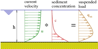


![{\displaystyle q_{ss}=<\int _{{z}_{a}}^{h\left(t\right)}{\left[u\left(z\right)c\left(z\right)+{\overline {u}}\left(z,t\right){\overline {c}}\left(z,t\right)\right]}dz>}](https://en.wikipedia.org/api/rest_v1/media/math/render/svg/fe2787c4bb03db6cbc108f29540c3fb96cc1bc48)


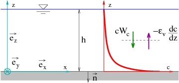


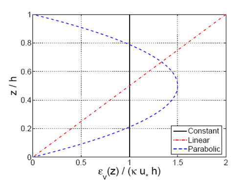
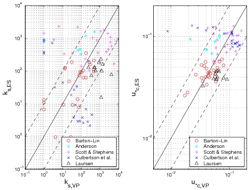
![{\displaystyle {{\varepsilon }_{c,i}}={\frac {-{{W}_{s}}c(i)}{\left\{c\left(i+1\right)-c\left(i-1\right)/\left[z\left(i+1\right)-z\left(i-1\right)\right]\right\}}}}](https://en.wikipedia.org/api/rest_v1/media/math/render/svg/68a91ad3f2c8b43ab9e4a5e26da7a30554288551)


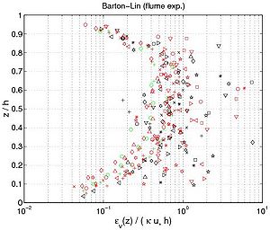
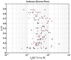
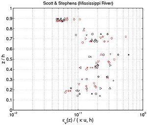
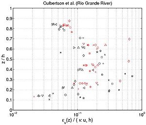
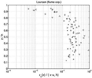
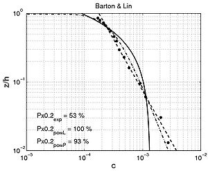
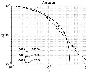
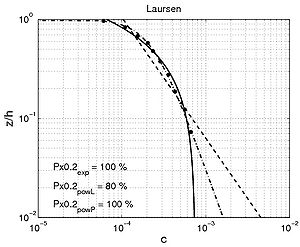
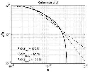
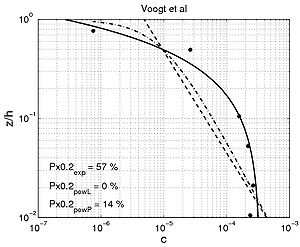
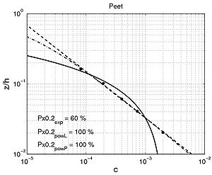
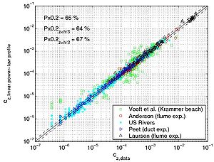

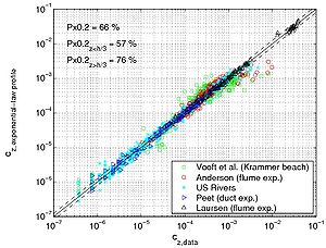


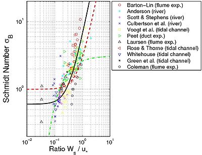


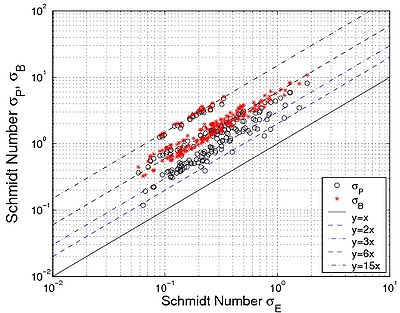

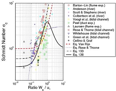


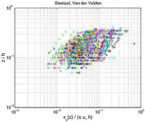
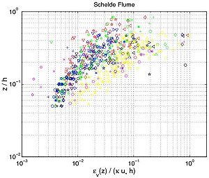
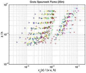
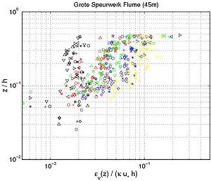
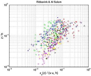
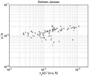
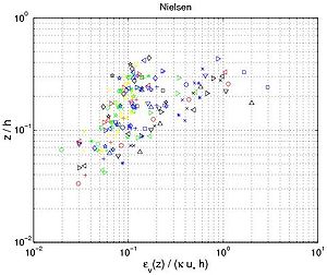
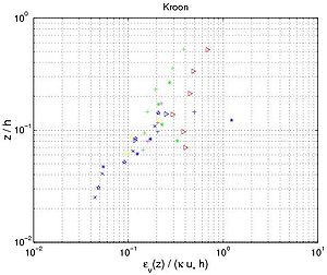
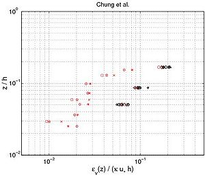
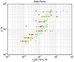
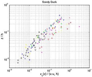
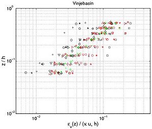
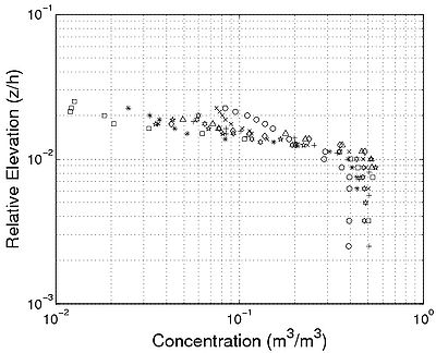
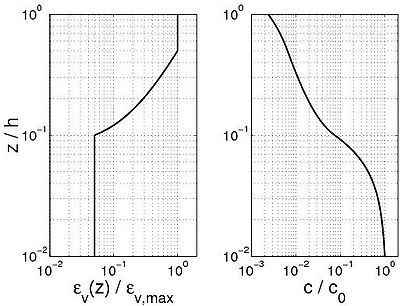
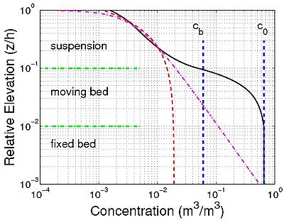
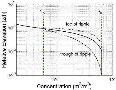
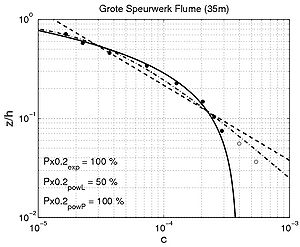
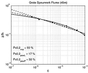
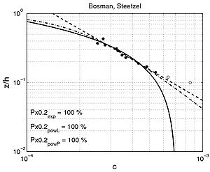
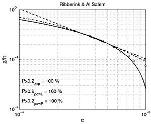
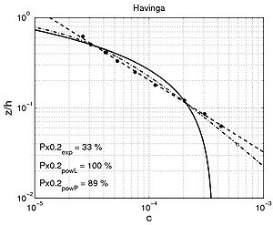
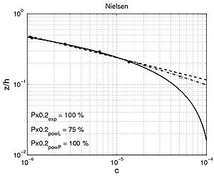
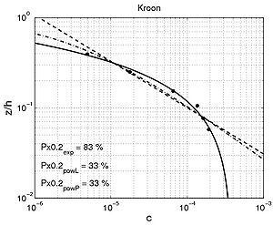
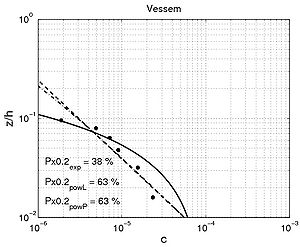
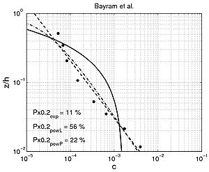
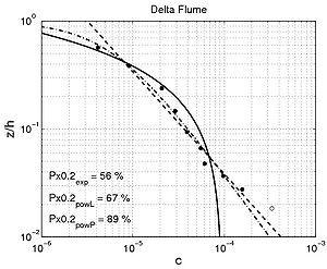
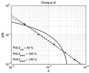
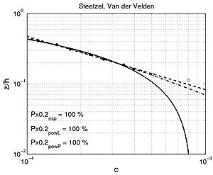
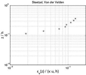
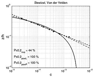
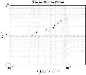
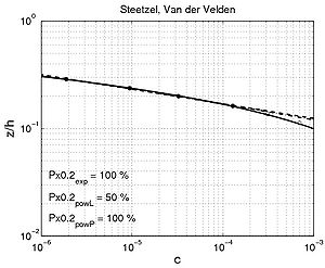
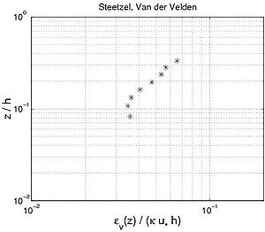
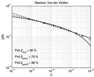
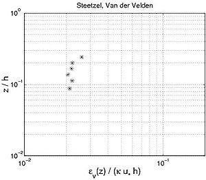


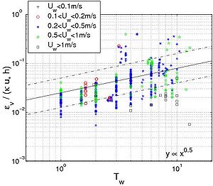
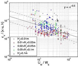
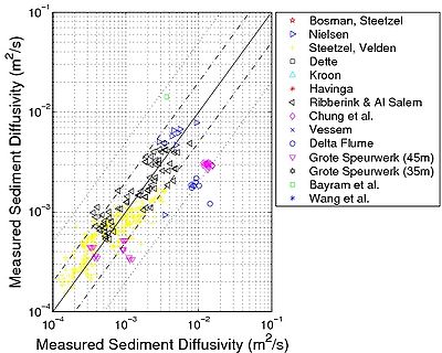


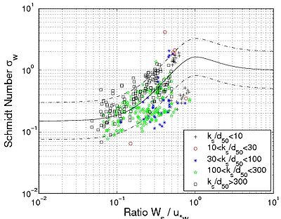

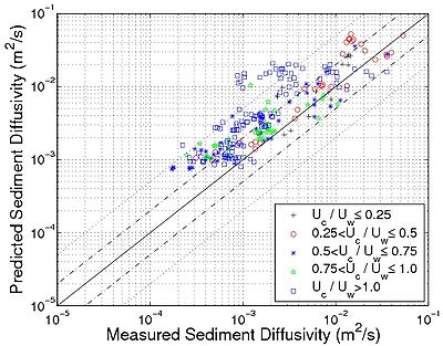


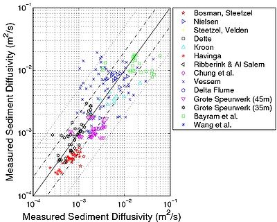


![{\displaystyle C_{g}={\frac {C}{2}}\left[1+{\frac {2k_{w}h}{\sinh(2k_{w}h)}}\right]}](https://en.wikipedia.org/api/rest_v1/media/math/render/svg/a9b77ad2593424eb83bd9c5fb59df5ebbacf25f1)


![{\displaystyle \alpha _{b}=\exp \left[-{\left({\frac {\gamma _{b}h}{H_{rms}}}\right)}^{2}\right]}](https://en.wikipedia.org/api/rest_v1/media/math/render/svg/04cbc136edc2a1a78932e67b88777e2201f1c2bb)
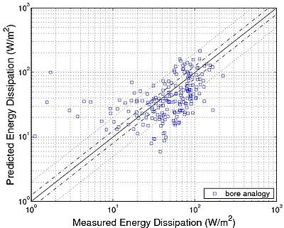

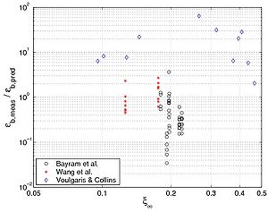
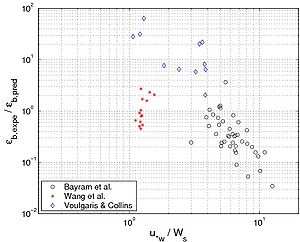
![{\displaystyle k_{b}=0.062\left[1-0.9\tanh \left(0.25{\frac {u_{*w}}{W_{s}}}\right)\right]}](https://en.wikipedia.org/api/rest_v1/media/math/render/svg/ccb7dd249b12400f1a3122328710ba324ff472d7)
![{\displaystyle k_{b}=0.012\left[1+1.0\tanh \left(\xi _{\infty }\right)\right]}](https://en.wikipedia.org/api/rest_v1/media/math/render/svg/ac7eff9d1577ff29ba35467e314bb2358d3ee56e)
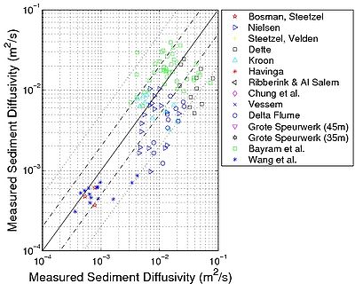

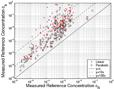

![{\displaystyle {\begin{aligned}&{\text{with }}\lambda =4.3{{\left({\frac {{{{\theta }'}_{c}}-{{\theta }_{cr}}-0.26p}{{{\theta }'}_{c}}}\right)}^{0.5}}\\&{\text{and }}p=\left[1+{{\left({\frac {0.26}{{{{\theta }'}_{c}}-{{\theta }_{cr}}}}\right)}^{4}}\right]-0.25\\\end{aligned}}}](https://en.wikipedia.org/api/rest_v1/media/math/render/svg/bd3a94d41ac7f7255e67df9abd5e6cbf245682c5)


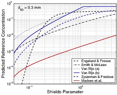


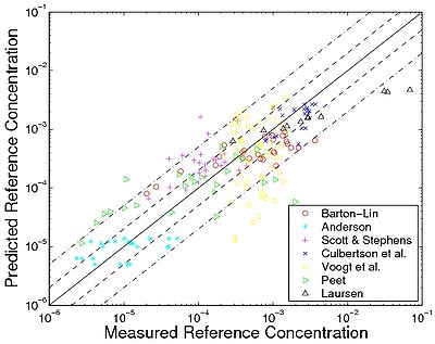


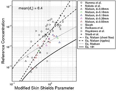

![{\displaystyle {{\theta }_{w,m}}={\frac {1}{{T}_{w}}}\int _{0}^{{T}_{w}}{1/2\ {{f}_{w}}\ u_{w}^{2}\left(t\right)/\left[\left(s-1\right)g{{d}_{50}}\right]dt}}](https://en.wikipedia.org/api/rest_v1/media/math/render/svg/a2e906de8a91c40c72e2a874da0fcb6f92c46a1a)


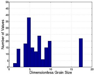
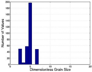
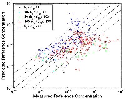
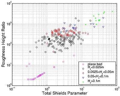


![{\displaystyle \theta _{cw,m}={\frac {1}{2}}{\frac {f_{cw}}{(s-1)gd_{50}}}\left[{\frac {1}{T_{w}}}\int _{0}^{Tw}\left(U_{c}\cos \varphi +u_{w}(t)\right)^{2}dt+\left(U_{c}\sin \varphi \right)^{2}\right]}](https://en.wikipedia.org/api/rest_v1/media/math/render/svg/b8b8ce50919a88ffc9ac1a77a1e86ee5317a2070)


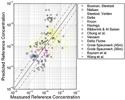
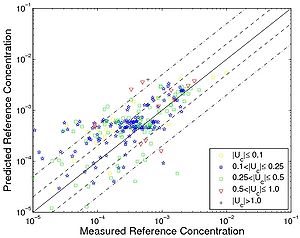
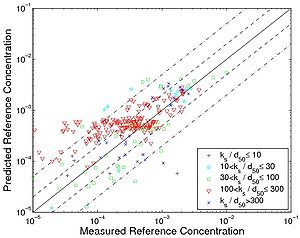
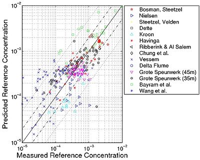
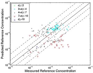
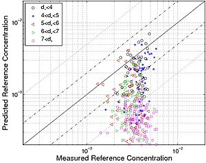
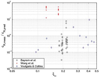
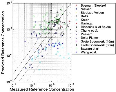
![{\displaystyle C_{Rb}=1.0+\tanh \left[50(\xi _{\infty }-0.15)\right]{\text{ if }}\xi _{\infty }>0.15}](https://en.wikipedia.org/api/rest_v1/media/math/render/svg/e351395b8c9ca98942c37e5997fff19537bf4849)


![{\displaystyle q_{ss}=1.83q_{sb}\left(I_{1}\ln \left[{\frac {33h}{\delta _{c}}}\right]+I_{2}\right)}](https://en.wikipedia.org/api/rest_v1/media/math/render/svg/1171bf57e241e3034a81abba284f3eb0c44efd87)


![{\displaystyle =U_{c}C_{R}{\frac {\varepsilon }{W_{s}}}\left[1-exp\ \left(-{\frac {W_{s}h}{\varepsilon }}\right)\right]}](https://en.wikipedia.org/api/rest_v1/media/math/render/svg/422545a53915e219c304f3e1874d4ebbf0ca1988)


![{\displaystyle c(t)=c_{0}[u(t+\phi _{pl})]^{2}}](https://en.wikipedia.org/api/rest_v1/media/math/render/svg/086e22a3806830d9317d268b3179ae15974fb10b)


![{\displaystyle \qquad ={\frac {r_{u}^{3}+r_{c}[1/2+X_{p}+r_{w}^{2}(2X_{p}^{2}-1/2)]+r_{w}/2(X_{p}^{2}+X_{p}-1/2)}{r_{u}^{3}+3/2r_{u}(1+r_{w}^{2})+3/4r_{w}}}}](https://en.wikipedia.org/api/rest_v1/media/math/render/svg/617c95369451af438b7fd9fff5af6ffda0a1e64f)


![{\displaystyle q_{ss,\phi _{pl}=0}={\frac {V_{c}+V_{t}}{U_{w}}}{\frac {1}{T_{w}}}\int _{0}^{T_{w}}c(t)dt={\frac {V_{c}+V_{t}}{U_{w}}}\left[r_{u}^{2}+{\frac {1}{2}}(1+r_{w}^{2})\right]}](https://en.wikipedia.org/api/rest_v1/media/math/render/svg/b872c0f5f2e2cb993f4d5e1238c8523a6ca5ae94)

![{\displaystyle q_{ss,net}={\frac {V_{c}(1-\alpha _{pl,s}+V_{t}(1+\alpha _{pl,s})}{U_{w}}}\left[r_{u}^{2}+{\frac {1}{2}}(1+r_{w}^{2})\right]}](https://en.wikipedia.org/api/rest_v1/media/math/render/svg/6fcfe4e1689832d2bfcfe10a41fb3d1b21360348)


}{r_{u}^{3}+3/2r_{u}(1+r_{w}^{2})+3/4r_{w}}}}](https://en.wikipedia.org/api/rest_v1/media/math/render/svg/f21f92f8dca3d035a016ec2e6bab9eb03de7cfdd)


![{\displaystyle \phi _{pl}=\pi \tanh \left[0.5\left({\frac {P_{WR}}{P_{WR,cr}}}\right)^{2}\right]}](https://en.wikipedia.org/api/rest_v1/media/math/render/svg/9b28a90420f427786e3d9577b4e5f2d9e5df47be)


![{\displaystyle \alpha _{pl,s}=(D_{pl,on}-D_{pl,off})\exp \left[-0.25\left({\frac {P_{WR,cr}}{P_{WR}}}\right)^{4}\right]}](https://en.wikipedia.org/api/rest_v1/media/math/render/svg/1d9962bf95fb9e86537574846290fbd3189e292f)


