Flat Basin: Difference between revisions
No edit summary |
No edit summary |
||
| (5 intermediate revisions by the same user not shown) | |||
| Line 77: | Line 77: | ||
|Coriolis force || Off | |Coriolis force || Off | ||
|} | |} | ||
The model is initialized from zero current velocities and water | |||
levels. The simulation is then allowed to reach steady state over | |||
48 hr. | |||
''Results and Discussion'' | |||
The calculated wind setup (water surface elevation) is shown in | |||
Figure 2 for the case of wind from the north (left) and from west | |||
(right). For both cases, the calculated wind setup is symmetric and | |||
has straight contour lines, which is consistent with the analytical | |||
solution. Figure 3 shows the wind setup along the center line of the | |||
domain for the case with wind from the north compared to the | |||
analytical solution. The goodness-of-fit statistics along this | |||
transect include the Normalized Root Mean Square Error (NRMSE), Mean | |||
Absolute Error (MAE), squared correlation coefficient,<math>R^2</math>, and | |||
Bias as given in Table 3. | |||
[[File:calculated_WL_IrregDom_a.png|left|thumb|400px|alt=framework]] | |||
[[File:calculated_WL_IrregDom_b.png||leftthumb|400px|alt=framework]] | |||
Figure 2. Calculated water levels in an irregular domain with a flat | |||
bed for the cases of wind from the north (left) and from the west | |||
(right). | |||
[[File:Analytical_and_Calculated_Water_Level_Profile.png||leftthumb|400px|alt=framework]] | |||
Figure 3. Analytical and calculated water level along the vertical | |||
centerline of an irregular basin with flat bed and winds from the | |||
south. The calculated results are shown on every 10th grid point for | |||
better visualization. | |||
Table 3. Water level goodness-of-fit statistics* for in the idealized | |||
wind setup test case. | |||
{| class="wikitable" border="1" | |||
|+ Table 2. CMS-Flow settings for the wind setup test case. | |||
! Statistic !! Value | |||
|- | |||
|NRMSE, % || 0.01 | |||
|- | |||
|NMAE, % || 0.02 | |||
|- | |||
|<math>R^2</math> || 0.999 | |||
|- | |||
|Bias, m || 0.000 | |||
|- | |||
*defined in Appendix A | |||
|} | |||
''Conclusions and Recommendations'' | |||
The steady wind set up in a closed basin with flat bed and irregular | |||
geometry was simulated and the model performance was measured using | |||
several goodness-of-fit statistics. The model accurately calculated | |||
the water level from wind setup with NRMSE of 0.01%, a NMAE of 0.02%, | |||
and <math>R^2</math> of 0.999. The test case demonstrated the model capability in | |||
simulating wind induced setup and verifies the implementation of both | |||
the wind driving force and water surface elevation terms. | |||
Latest revision as of 20:45, 15 April 2014
Test C1-Ex1: Wind Setup in a Flat Basin
Purpose
This verification test is designed to test the most basic model capabilities by solving the most reduced or simplified form of the governing equations in which only the water level gradient balances the wind surface drag. The specific model features/aspects to be tested are (1) spatially constant wind fields, (2) water surface gradient implementation, and (3) land-water boundary condition.
Problem and Analytical Solution
Assuming a closed basin with a spatially constant, steady state wind in one direction, no advection, diffusion, bottom friction, waves or Coriolis force, the momentum equations reduce to
| (1) |
where is the total water depth, is the
still water depth, is the water surface elevation (water
level) with respect to the still water level, is the wind drag
coefficient, is the coordinate in the direction of the wind,
is the gravitational acceleration, is the water
density, is the air density, and is the wind
speed. Assuming a constant wind drag coefficient, the following
analytical expression for the water level may be obtained by
integrating the above equation (Dean and Dalrymple 1984)
| (2) |
where is a constant of integration.
Model Setup
A computational grid with constant water depth of 5 m and irregular boundaries is used to verify the numerical methods. The computational grid has 60 columns and 70 rows and a constant resolution of 500 m. The irregular geometry is intentionally used to check for any discontinuities in processes near the land-water boundaries. The solution should be perfectly symmetric and independent of the geometry of the closed basin. The steady state solution is reached by increasing the wind speed over a 3 hr ramp period and allowing the solution to reach steady state over a 48 hr time period. During the ramp period, all model forcing is slowly increased from the initial condition (not necessarily zero), to the specified boundary condition time series. The purpose of the ramp period is to allow the model to slowly adjust to the forcing conditions without “shocking” it with a step function. In CMS, a cosine ramp function of the form
| (3) |
| Parameter | Value |
|---|---|
| Solution scheme | Implicit |
| Time step | 10 min |
| Simulation duration | 48 hr |
| Ramp period duration | 3 hr |
| Wind speed | 10 m/s |
| Drag coefficient | 0.0016 |
| Advection terms | Off |
| Mixing terms | Off |
| Bottom friction | Off |
| Wall friction | Off |
| Coriolis force | Off |
The model is initialized from zero current velocities and water levels. The simulation is then allowed to reach steady state over 48 hr.
Results and Discussion
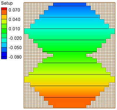
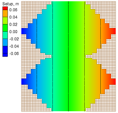
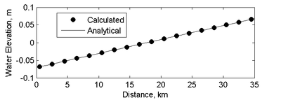
The calculated wind setup (water surface elevation) is shown in Figure 2 for the case of wind from the north (left) and from west (right). For both cases, the calculated wind setup is symmetric and has straight contour lines, which is consistent with the analytical solution. Figure 3 shows the wind setup along the center line of the domain for the case with wind from the north compared to the analytical solution. The goodness-of-fit statistics along this transect include the Normalized Root Mean Square Error (NRMSE), Mean Absolute Error (MAE), squared correlation coefficient,, and Bias as given in Table 3.

 Figure 2. Calculated water levels in an irregular domain with a flat
bed for the cases of wind from the north (left) and from the west
(right).
 Figure 3. Analytical and calculated water level along the vertical
centerline of an irregular basin with flat bed and winds from the
south. The calculated results are shown on every 10th grid point for
better visualization.
Table 3. Water level goodness-of-fit statistics* for in the idealized wind setup test case.
- defined in Appendix A
| Statistic | Value |
|---|---|
| NRMSE, % | 0.01 |
| NMAE, % | 0.02 |
| 0.999 | |
| Bias, m | 0.000 |
Conclusions and Recommendations
The steady wind set up in a closed basin with flat bed and irregular geometry was simulated and the model performance was measured using several goodness-of-fit statistics. The model accurately calculated the water level from wind setup with NRMSE of 0.01%, a NMAE of 0.02%, and of 0.999. The test case demonstrated the model capability in simulating wind induced setup and verifies the implementation of both the wind driving force and water surface elevation terms.