Li: Difference between revisions
No edit summary |
No edit summary |
||
| (5 intermediate revisions by the same user not shown) | |||
| Line 1: | Line 1: | ||
= Purpose = | |||
Application of CMS to the Gironde Estuary demonstrates specification | |||
of the flow boundary condition within an estuary, with validation | |||
measurements of water level and current speed spaced along the axis of | |||
the estuary. | |||
= Field Study = | |||
The Gironde Estuary is located in southwestern France. It receives | |||
runoff from the Garonne and the Dordogne Rivers and opens up to the | |||
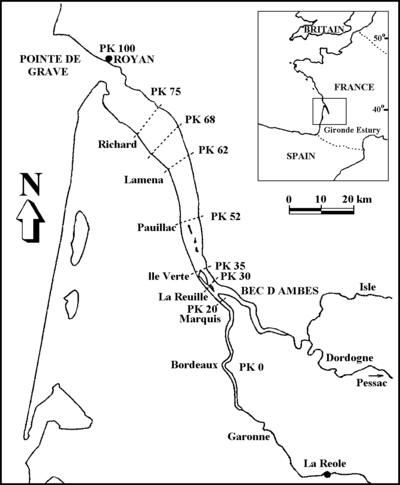
Atlantic Ocean, as shown in Figure 1. The water-surface width varies | |||
from 2 to 14 km, and the flow depth in the navigation channel ranges | |||
from 6 to 30 m. The estuary is partially mixed and macrotidal, with a | |||
12 hr and 25 min tidal lunar period and a tidal amplitude of 1.5 to | |||
5 m at the mouth (Li et al. 1994). | |||
[[File:Gironde_Estuary.png |thumb|right|400px|Figure 1. Sketch of the Gironde Estuary, France (from Wu and Wang 2004).]] | |||
= Model Setup = | |||
| | |||
| | The implicit CMS was applied to this test case, with the simulation | ||
| | domain extending 80 km starting from the mouth at the Atlantic Ocean | ||
| | to the Garonne and Dordogne Rivers. The bed topography was provided on | ||
| | a uniform mesh, with a size of 250 × 125 m for each cell. The grid has | ||
|- | approximately 16,000 active cells. Because the domain is relatively | ||
| | simple, a uniform mesh was used. The data measured from May 19 to 25, | ||
|- | 1975 were used to validate the model for water level and current | ||
| | speed. The computational time step was set to 30 min. At the estuary | ||
|- | mouth, the tidal elevation was given by the recorded time series at | ||
| | the station “Pointe de Grave” (see Figure 1). At the two upstream | ||
|- | ends, the flow discharges of the Garonne River and the Dordogne River | ||
were specified according to the measured data at La Réole and | |||
Pessac. The Manning’s roughness coefficient was set to | |||
0.018 s/m1/3. Figure 2 shows the computational grid and observation | |||
stations. The Coriolis force is included using the f-plane | |||
approximation. Winds were not included in the simulation. The 100-hr | |||
simulation took approximately 12 min to run on a 2.67 GHz processor. | |||
[[File:Gironde_Estuary_Computational_Grid.png |thumb|right|400px|Figure 2. Computational grid and observation stations for the Gironde Estuary Test Case.]] | |||
The inland boundaries along the Dordogne and Garonne rivers were | |||
assigned as flux boundary conditions according to the data from La | |||
Réole and Pessac, and the inflow discharges were set to 387 and | |||
846 m3/s, respectively. The initial condition was specified as still | |||
water in the whole domain. A 1-hr ramp period was used at the start | |||
the simulation. Table 1 summarizes the setup parameters for CMS. | |||
{| border="1" | |||
|+ Table 1. CMS-Flow setup parameters for the Gironde Estuary test case. | |||
!Parameter !!Value | |||
|- | |||
|Solution scheme ||Implicit | |||
|- | |||
|Simulation duration ||100 hr | |||
|- | |||
|Ramp period duration ||1 hr | |||
|- | |||
|Time step ||6 min | |||
|- | |||
|Manning’s n coefficient ||0.018 s/m1/3 | |||
|- | |||
|Latitude ||45.5° | |||
|} | |||
= Results and Discussion = | |||
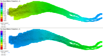
The flow fields in flood and ebb tides are shown in Figure 3. The ebb | |||
flow is characterized by a funnel effect at the entrance (mouth or | |||
inlet) caused by the narrowing of the estuary in this region. The | |||
increase in velocity is likely to be the cause of the channel | |||
deepening in this region as shown by the depth contours (see | |||
Figure 2). The flood tide is also characterized by a funnel effect | |||
near Ile Verte which also seems to cause some deepening of the estuary | |||
to the south of the island. | |||
[[File:Gironde_Currents.png |thumb|right|400px|Figure 3. Examples of ebb (top) and flood (bottom) tidal currents and water surface elevations in the Gironde Estuary.]] | |||
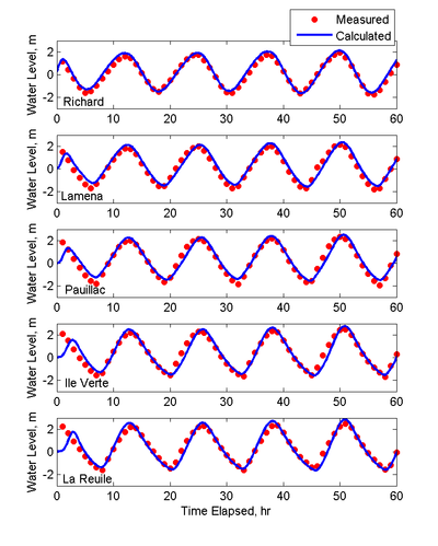
Figure 4 compares the measured and simulated water levels at five | |||
stations within the Gironde Estuary (stations shown in Figure 2). In | |||
general, the results show good agreement with the measured data both | |||
in amplitude and phase. Table 2 summarizes the goodness–of-fit | |||
statistics for water level. NRMSE and NMAE values for the water levels | |||
range from 5-7%. | |||
[[File:Gironde_Water_Levels.png |thumb|right|400px|Figure 4. Comparison of measured and calculated water levels at five stations in the Gironde Estuary (stations shown in Figure 2).]] | |||
{| border="1" | |||
|+ Table 2. Water level goodness-of-fit statistics* for the Gironde Estuary test case. | |||
!Statistic !!Richard !!Lamena !!Pauillac !!Ile Verte !!La Reuille | |||
|- | |||
|NRMSE, % ||5.10 ||7.02 ||6.74 ||6.40 ||6.63 | |||
|- | |||
|NMAE, % ||4.33 ||6.21 ||5.63 ||4.34 ||5.08 | |||
|- | |||
|<math>R^2</math> ||0.982 ||0.956 ||0.951 ||0.962 ||0.972 | |||
|- | |||
|Bias, m ||0.094 ||0.128 ||0.043 ||-0.060 ||-0.0252 | |||
|} | |||
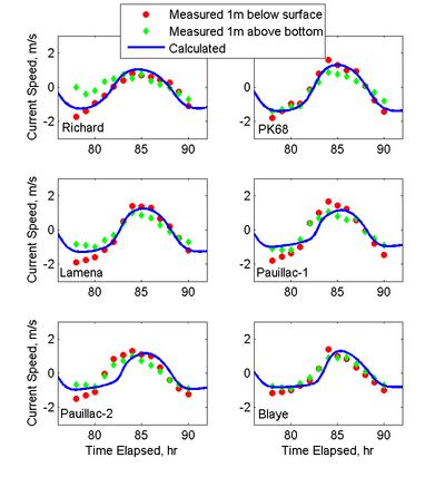
Figure 5 shows the comparison of the measured and simulated flow | |||
velocities at several stations (stations shown in Figure 2). The | |||
velocities were measured 1 m below the water surface and 1 m above the | |||
river bed, respectively. In this figure, positive current velocities | |||
correspond to flood tides and negative velocities to ebb tides. The | |||
current measurements at both elevations are relatively similar for all | |||
stations except Richard and Lamena. This might be due to baroclinic | |||
circulation produced by wind, fresh water intrusion, or other factors | |||
near these two stations. | |||
Some of the differences in water surface elevations and current | |||
velocities may be due to inaccuracies in the boundary conditions. The | |||
boundary conditions at the estuary entrance was obtained from a nearby | |||
station and therefore a slight phase lag of about 45 min was | |||
subtracted from calculated water surface elevations in order to match | |||
the measured time series. However, since the boundary condition used | |||
was not measured exactly at the location of the boundary, some error | |||
in phase lag may be expected from this approximation. | |||
Another probable source of error is the bottom roughness coefficient, | |||
which was assumed to be constant. Other field experiments show that | |||
the bottom roughness in an estuary can vary significantly due to | |||
changes in bed forms and grain sizes within the estuary. Although the | |||
CMS has the capability to use a spatially variable bottom roughness | |||
coefficient, there were no data available in this case. The agreement | |||
between measured and calculated current speeds is summarized in | |||
Table 3. NRMSE and NMAE in current speed range from 7-21%. Comparable | |||
results were obtained by Wu and Wang (2004) using a similar | |||
depth-averaged flow model. | |||
[[File:Gironde_Current_Speed.png |thumb|right|400px|Figure 5. Measured and calculated current speed in the Gironde Estuary (stations shown in Figure 2) ]] | |||
{| border="1" | |||
|+ Table 3. Current speed goodness of fit statistics for the Gironde Estuary test case. | |||
!Statistic !!Richard !!PK68 !!Lamena !!Pauillac-1 !!Pauillac-2 !!Blaye | |||
|- | |||
|NRMSE, % ||10.70 ||7.27 ||8.81 ||15.89 ||20.73 ||14.98 | |||
|- | |||
|NMAE, % ||9.15 ||5.71 ||6.93 ||13.67 ||17.05 ||13.17 | |||
|- | |||
|R2 ||0.911 ||0.957 ||0.968 ||0.856 ||0.680 ||0.804 | |||
|- | |||
|Bias, m/s ||0.070 ||-0.057 ||0.062 ||0.022 ||-0.031 ||0.095 | |||
|} | |} | ||
= Conclusions and Recommendations = | |||
CMS calculations of tidal flow in a large estuary were compared to | |||
measured water level and current speed. Calculations agreed with | |||
measurements with errors ranging from 5-7% for water level and 7-21% | |||
for currents. The boundary condition used in the model was not | |||
measured exactly at the location of the boundary, and therefore the | |||
calculations incurred some error in phase lag of water surface | |||
elevation and in current velocities. This application demonstrates | |||
the accuracy of CMS within a macrotidal estuarine environment, for | |||
measurements distributed along the channel. It is recommended that the | |||
bottom roughness be estimated based on the bottom type (sandy, rocky | |||
outcrops, vegetation, etc.), and then adjusted (calibrated) based on | |||
field measurements of water levels and currents. When developing a new | |||
model setup and grid for engineering applications, it is useful to | |||
start simple as far as grid size and model forcing, and slow increase | |||
the model complexity, only as needed until satisfactory results are | |||
obtained for the purpose of the project. This iterative process has | |||
the added benefit of providing insights on the importance of physical | |||
processes and model sensitivity to setup parameters and grid geometry. | |||
= References = | |||
* Li, Z.H., Nguyen, K.D., Brun-Cottan, J.C. and Martin, J.M., (1994). “Numerical simulation of the turbidity maximum transport in the Gironde Estuary (France)” Oceanologica Acta, 17(5), 479–500. | |||
* Wu, W., and Wang, S.S.Y. (2004). “Depth-averaged 2-D calculation of tidal flow, salinity and cohesive sediment transport in estuaries.” International Journal of Sediment Research, 19(3), 172-190. | |||
---- | |||
[[Test_Cases]] | |||
Latest revision as of 17:05, 23 April 2014
Purpose
Application of CMS to the Gironde Estuary demonstrates specification of the flow boundary condition within an estuary, with validation measurements of water level and current speed spaced along the axis of the estuary.
Field Study
The Gironde Estuary is located in southwestern France. It receives runoff from the Garonne and the Dordogne Rivers and opens up to the Atlantic Ocean, as shown in Figure 1. The water-surface width varies from 2 to 14 km, and the flow depth in the navigation channel ranges from 6 to 30 m. The estuary is partially mixed and macrotidal, with a 12 hr and 25 min tidal lunar period and a tidal amplitude of 1.5 to 5 m at the mouth (Li et al. 1994).

Model Setup
The implicit CMS was applied to this test case, with the simulation domain extending 80 km starting from the mouth at the Atlantic Ocean to the Garonne and Dordogne Rivers. The bed topography was provided on a uniform mesh, with a size of 250 × 125 m for each cell. The grid has approximately 16,000 active cells. Because the domain is relatively simple, a uniform mesh was used. The data measured from May 19 to 25, 1975 were used to validate the model for water level and current speed. The computational time step was set to 30 min. At the estuary mouth, the tidal elevation was given by the recorded time series at the station “Pointe de Grave” (see Figure 1). At the two upstream ends, the flow discharges of the Garonne River and the Dordogne River were specified according to the measured data at La Réole and Pessac. The Manning’s roughness coefficient was set to 0.018 s/m1/3. Figure 2 shows the computational grid and observation stations. The Coriolis force is included using the f-plane approximation. Winds were not included in the simulation. The 100-hr simulation took approximately 12 min to run on a 2.67 GHz processor.

The inland boundaries along the Dordogne and Garonne rivers were
assigned as flux boundary conditions according to the data from La
Réole and Pessac, and the inflow discharges were set to 387 and
846 m3/s, respectively. The initial condition was specified as still
water in the whole domain. A 1-hr ramp period was used at the start
the simulation. Table 1 summarizes the setup parameters for CMS.
| Parameter | Value |
|---|---|
| Solution scheme | Implicit |
| Simulation duration | 100 hr |
| Ramp period duration | 1 hr |
| Time step | 6 min |
| Manning’s n coefficient | 0.018 s/m1/3 |
| Latitude | 45.5° |
Results and Discussion
The flow fields in flood and ebb tides are shown in Figure 3. The ebb flow is characterized by a funnel effect at the entrance (mouth or inlet) caused by the narrowing of the estuary in this region. The increase in velocity is likely to be the cause of the channel deepening in this region as shown by the depth contours (see Figure 2). The flood tide is also characterized by a funnel effect near Ile Verte which also seems to cause some deepening of the estuary to the south of the island.

Figure 4 compares the measured and simulated water levels at five stations within the Gironde Estuary (stations shown in Figure 2). In general, the results show good agreement with the measured data both in amplitude and phase. Table 2 summarizes the goodness–of-fit statistics for water level. NRMSE and NMAE values for the water levels range from 5-7%.

| Statistic | Richard | Lamena | Pauillac | Ile Verte | La Reuille |
|---|---|---|---|---|---|
| NRMSE, % | 5.10 | 7.02 | 6.74 | 6.40 | 6.63 |
| NMAE, % | 4.33 | 6.21 | 5.63 | 4.34 | 5.08 |
| 0.982 | 0.956 | 0.951 | 0.962 | 0.972 | |
| Bias, m | 0.094 | 0.128 | 0.043 | -0.060 | -0.0252 |
Figure 5 shows the comparison of the measured and simulated flow velocities at several stations (stations shown in Figure 2). The velocities were measured 1 m below the water surface and 1 m above the river bed, respectively. In this figure, positive current velocities correspond to flood tides and negative velocities to ebb tides. The current measurements at both elevations are relatively similar for all stations except Richard and Lamena. This might be due to baroclinic circulation produced by wind, fresh water intrusion, or other factors near these two stations.
Some of the differences in water surface elevations and current velocities may be due to inaccuracies in the boundary conditions. The boundary conditions at the estuary entrance was obtained from a nearby station and therefore a slight phase lag of about 45 min was subtracted from calculated water surface elevations in order to match the measured time series. However, since the boundary condition used was not measured exactly at the location of the boundary, some error in phase lag may be expected from this approximation.
Another probable source of error is the bottom roughness coefficient, which was assumed to be constant. Other field experiments show that the bottom roughness in an estuary can vary significantly due to changes in bed forms and grain sizes within the estuary. Although the CMS has the capability to use a spatially variable bottom roughness coefficient, there were no data available in this case. The agreement between measured and calculated current speeds is summarized in Table 3. NRMSE and NMAE in current speed range from 7-21%. Comparable results were obtained by Wu and Wang (2004) using a similar depth-averaged flow model.

| Statistic | Richard | PK68 | Lamena | Pauillac-1 | Pauillac-2 | Blaye |
|---|---|---|---|---|---|---|
| NRMSE, % | 10.70 | 7.27 | 8.81 | 15.89 | 20.73 | 14.98 |
| NMAE, % | 9.15 | 5.71 | 6.93 | 13.67 | 17.05 | 13.17 |
| R2 | 0.911 | 0.957 | 0.968 | 0.856 | 0.680 | 0.804 |
| Bias, m/s | 0.070 | -0.057 | 0.062 | 0.022 | -0.031 | 0.095 |
Conclusions and Recommendations
CMS calculations of tidal flow in a large estuary were compared to measured water level and current speed. Calculations agreed with measurements with errors ranging from 5-7% for water level and 7-21% for currents. The boundary condition used in the model was not measured exactly at the location of the boundary, and therefore the calculations incurred some error in phase lag of water surface elevation and in current velocities. This application demonstrates the accuracy of CMS within a macrotidal estuarine environment, for measurements distributed along the channel. It is recommended that the bottom roughness be estimated based on the bottom type (sandy, rocky outcrops, vegetation, etc.), and then adjusted (calibrated) based on field measurements of water levels and currents. When developing a new model setup and grid for engineering applications, it is useful to start simple as far as grid size and model forcing, and slow increase the model complexity, only as needed until satisfactory results are obtained for the purpose of the project. This iterative process has the added benefit of providing insights on the importance of physical processes and model sensitivity to setup parameters and grid geometry.
References
- Li, Z.H., Nguyen, K.D., Brun-Cottan, J.C. and Martin, J.M., (1994). “Numerical simulation of the turbidity maximum transport in the Gironde Estuary (France)” Oceanologica Acta, 17(5), 479–500.
- Wu, W., and Wang, S.S.Y. (2004). “Depth-averaged 2-D calculation of tidal flow, salinity and cohesive sediment transport in estuaries.” International Journal of Sediment Research, 19(3), 172-190.