User Guide 002: Difference between revisions
No edit summary |
No edit summary |
||
| (48 intermediate revisions by the same user not shown) | |||
| Line 4: | Line 4: | ||
The CMS-Flow (and also for most morphodynamic models) input and output can be classified as: | The CMS-Flow (and also for most morphodynamic models) input and output can be classified as: | ||
1. Input | :1. Input | ||
a. Control file (model parameters, options, pointers to other files). | |||
b. Geometry (grid). | ::a. Control file (model parameters, options, pointers to other files). | ||
c. Initial condition (bathymetry, bed composition, etc.). | |||
d. Boundary conditions | ::b. Geometry (grid). | ||
2. Output | |||
a. Transient solution | ::c. Initial condition (bathymetry, bed composition, etc.). | ||
i. Global (for the whole domain) | |||
ii. Point (at a single point or cell) | ::d. Boundary conditions | ||
b. Statistical parameters | |||
c. Hot start (may include internal variables) | :2. Output | ||
d. Diagnostic Files | |||
::a. Transient solution | |||
:::i. Global (for the whole domain) | |||
:::ii. Point (at a single point or cell) | |||
::b. Statistical parameters | |||
::c. Hot start (may include internal variables) | |||
::d. Diagnostic Files | |||
A detailed description of the CMS input and output files is provided below. | A detailed description of the CMS input and output files is provided below. | ||
| Line 21: | Line 32: | ||
==Input Files== | ==Input Files== | ||
There are at least three required files to run CMS-Flow: (1) the ''Card File'' (*.cmcards), (2) the ''XMDF Grid File'' (*_grid.h5), (3) and the ''XMDF Model Parameters File''. If a telescoping grid is used then an additional ASCII ''Telescoping Grid File'' is required. For a description of types of Cartesian grids available in CMS-Flow see section | There are at least three required files to run CMS-Flow: (1) the ''Card File'' (*.cmcards), (2) the ''XMDF Grid File'' (*_grid.h5), (3) and the ''XMDF Model Parameters File''. If a telescoping grid is used then an additional ASCII ''Telescoping Grid File'' is required. For a description of types of Cartesian grids available in CMS-Flow see section <span style="color:#0000FF">Cartesian Grids</span>. If any input datasets such as the Manning’s coefficient or bed composition are specified in separate XMDF files then the file name and path must be specified in the ''Card File''. Using separate input files for user-defined datasets makes it easier to make project alternatives or conduct sensitivity studies. The user-defined datasets can be easily created and exported from SMS. The procedure is described in detail in subsequent sections. A brief description of the CMS input files is provided in the table below. | ||
Table 2-1. CMS-Flow Input Files | |||
{| class="wikitable" | |||
|- | |||
!File | |||
!Name | |||
!Description | |||
|- | |||
|Card File | |||
|*.cmcards | |||
|File name including path for the CMS-Wave sim file. | |||
|- | |||
|XMDF Grid File | |||
|*_grid.h5 | |||
|Specifies the coordinates, and depths of the CMS-Flow grid(s). If a telescoping grid is used, multiple grids are saved for each refinement level. | |||
|- | |||
|XMDF Model Parameters File | |||
|*_mp.h5 | |||
|Specifies boundary forcing information, wind forcing, and geographical coordinates. | |||
|- | |||
|Telescoping Grid File | |||
|*.tel | |||
|Specifies the cell coordinates, dimensions, and depths for the telescoping grid file. Only saved in the case a telescoping grid is used. | |||
|- | |||
|User-defined Dataset Files | |||
|*.h5 | |||
|Determines the extrapolation distance used for flow variables on the wave grid. | |||
|} | |||
==CMS-Flow Card/Control File== | ==CMS-Flow Card/Control File== | ||
| Line 29: | Line 67: | ||
In CMS-Flow, the ''Control File'' is an ASCII text file referred to also as the ''Card File'' because it contains a list of cards used to specify model input such as parameters, coefficients, options, etc. A card is simply a unique character string which the model uses to identify a specific model input. The ''Card File'' is the main input file which sets input parameters and points to other files. In general most of the “light” input data is specified in the ''Card File''. Light data refers to input parameters which is relatively small in size and can easily be specified by the user in a few lines such as global parameters. Any input that is relatively large, such as time series, and spatially varying datasets are referred to as “heavy” data. Heavy data is stored in separate files such as the ''Grid File, Model Parameters File'', or other user-specified files. The heavy data is then simply pointed to in the ''Card File''. | In CMS-Flow, the ''Control File'' is an ASCII text file referred to also as the ''Card File'' because it contains a list of cards used to specify model input such as parameters, coefficients, options, etc. A card is simply a unique character string which the model uses to identify a specific model input. The ''Card File'' is the main input file which sets input parameters and points to other files. In general most of the “light” input data is specified in the ''Card File''. Light data refers to input parameters which is relatively small in size and can easily be specified by the user in a few lines such as global parameters. Any input that is relatively large, such as time series, and spatially varying datasets are referred to as “heavy” data. Heavy data is stored in separate files such as the ''Grid File, Model Parameters File'', or other user-specified files. The heavy data is then simply pointed to in the ''Card File''. | ||
Example 2 1. CMS-Flow Cards. | Example 2-1. CMS-Flow Cards. | ||
---- | |||
---- | |||
<span style="color:#0000FF">CMS_VERSION</span> 4.0 <span style="color:#008000">!Version of input card file</span> | <span style="color:#0000FF">CMS_VERSION</span> 4.0 <span style="color:#008000">!Version of input card file</span> | ||
| Line 38: | Line 78: | ||
<span style="color:#0000FF">TIME_LIST_1 </span> 2 0.0 3.0 1.0 3.0 6.0 0.5 | <span style="color:#0000FF">TIME_LIST_1 </span> 2 0.0 3.0 1.0 3.0 6.0 0.5 | ||
---- | |||
---- | |||
| Line 45: | Line 87: | ||
The CMS-Flow Card File is a simple ASCII file with the following simple formatting rules and conventions: | The CMS-Flow Card File is a simple ASCII file with the following simple formatting rules and conventions: | ||
1. Commented lines should be preceded by the characters ! or # or ignored. Comments can start at any column within the card file. | :1. Commented lines should be preceded by the characters ! or # or ignored. Comments can start at any column within the card file. | ||
2. Cards are always written in capital letters. | :2. Cards are always written in capital letters. | ||
3. Any character string in all capital letters after a card is an argument from a list options for that specific card (e.g. ON or OFF). | :3. Any character string in all capital letters after a card is an argument from a list options for that specific card (e.g. <span style="color:#FF0000">ON</span> or <span style="color:#FF0000">OFF</span>). | ||
4. Card arguments are read in free-format. This means that input arguments should always be separated by at least one blank space or a comma. | :4. Card arguments are read in free-format. This means that input arguments should always be separated by at least one blank space or a comma. | ||
5. Cards should always begin on a new line (i.e. only one card is allowed per line). | :5. Cards should always begin on a new line (i.e. only one card is allowed per line). | ||
6. Character strings do not need to be enclosed in single or double quotation unless they contain white spaces. No characters besides letters (no accents) and numbers are allowed in character strings except: ‘(’, ‘)’, and ‘-’. | :6. Character strings do not need to be enclosed in single or double quotation unless they contain white spaces. No characters besides letters (no accents) and numbers are allowed in character strings except: ‘(’, ‘)’, and ‘-’. | ||
7. The end of the card file is specified by the END_PARAMETERS card. Any statements after this card are ignored. | :7. The end of the card file is specified by the <span style="color:#0000FF">END_PARAMETERS</span> card. Any statements after this card are ignored. | ||
==Style Recommendations== | ==Style Recommendations== | ||
| Line 63: | Line 105: | ||
The following recommendations are optional and provided for readability and to avoid commonly made formatting errors. | The following recommendations are optional and provided for readability and to avoid commonly made formatting errors. | ||
1. Single line cards should start at the first column unless the card is specified within a block in which case the card should be indented by 2 to 3 spaces. | :1. Single line cards should start at the first column unless the card is specified within a block in which case the card should be indented by 2 to 3 spaces. | ||
:2. Input arguments should start at column 37 for readability. | |||
:3. Double quotes should be used for file names and paths | |||
:4. Single quotes should be used for units. | |||
Table 2-2. CMS-Flow Card notation. | |||
{| class="wikitable" | |||
!Notation | |||
!Description | |||
|- | |||
|! | |||
|Indicates the beginning of a comment. Comments may begin at any column. Recommended for inserting headers and comments. | |||
|- | |||
|# | |||
|Indicates to ignore the rest of a line. Recommended for commenting cards. | |||
|- | |||
|ON | |||
|Activates a model feature | |||
|- | |||
|OFF | |||
|Deactivates a model feature | |||
|- | |||
|“ ” | |||
|Indicates a character string such as a file name or path | |||
|- | |||
|‘ ’ | |||
|Indicates a character string for input argument units such as ‘m^3/s’ | |||
|} | |||
Many input cards have relationships to one another. For example a card may only be applicable if another card is specified. This is referred to here as a dependency. Dependencies are hierarchal in nature and may be listed either downwards or upwards in the dependency tree. One example of a dependency is the angle and repose and avalanching activation cards. The angle of repose is dependent on the avalanching being activated; otherwise it is not applicable. When two cards cannot exist together because they conflict with one another, this is referred to as an exclusion. An example of an exclusion is the bottom roughness specification using both a Manning’s n and bottom friction coefficient. The bottom roughness can only be specified once and therefore the input cards used to specify the Manning’s and bottom friction coefficient would conflict with one another. In the tables describing the input cards it is convenient to use to establish a notation for the card input formats. | Many input cards have relationships to one another. For example a card may only be applicable if another card is specified. This is referred to here as a dependency. Dependencies are hierarchal in nature and may be listed either downwards or upwards in the dependency tree. One example of a dependency is the angle and repose and avalanching activation cards. The angle of repose is dependent on the avalanching being activated; otherwise it is not applicable. When two cards cannot exist together because they conflict with one another, this is referred to as an exclusion. An example of an exclusion is the bottom roughness specification using both a Manning’s n and bottom friction coefficient. The bottom roughness can only be specified once and therefore the input cards used to specify the Manning’s and bottom friction coefficient would conflict with one another. In the tables describing the input cards it is convenient to use to establish a notation for the card input formats. | ||
Table 2-3. CMS-Flow Card format operators. | |||
{|class="wikitable" | |||
|- | |||
!Notation | |||
!Description | |||
|- | |||
|[] | |||
|Indicates a required input value (card or argument) | |||
|- | |||
|< | |||
|Specifies the range of an argument to be less than a value | |||
|- | |||
|> | |||
|Specifies the range of an argument to be greater than a value | |||
|- | |||
|<= | |||
|Specifies the range of an argument to be less or equal to a value | |||
|- | |||
|> | |||
|Specifies the range of an argument to be greater or equal to a value | |||
|- | |||
|= | |||
|Specifies the value(s) of an input argument | |||
|} | |||
Table 2-4. CMS-Flow Card Format key word description. | |||
{|class="wikitable" | |||
|- | |||
!Notation | |||
!Description | |||
|- | |||
|begin | |||
|Block structure begin statement | |||
|- | |||
|end | |||
|Block structure end statement | |||
|- | |||
|card | |||
|Character string for a card | |||
|- | |||
|arg | |||
|Variable name for a card argument | |||
|- | |||
|units | |||
|Unit type for input argument (generally optional) | |||
|- | |||
|options | |||
|List of card argument options | |||
|- | |||
|type | |||
|Argument type as floating (float), integer (int), or character (char) | |||
|- | |||
|float | |||
|Argument type as a real or floating | |||
|- | |||
|int | |||
|Argument type as an integer | |||
|- | |||
|char | |||
|Argument type as a character string | |||
|- | |||
|limits | |||
|Limits of the input argument if they exist | |||
|- | |||
|default | |||
|Argument default value if it exists. If an automatic default value is available then the automatic mode can be used. | |||
|- | |||
|dependencies | |||
|List of cards for which there exist a dependency | |||
|- | |||
|exclusions | |||
|List of cards for which there exist an exclusion | |||
|- | |||
|symbol | |||
|Mathematical symbol used for an input argument | |||
|- | |||
|required | |||
|Indicates whether in input argument is required or not | |||
|- | |||
|typical | |||
|Specifies a typical value or range for an input card. | |||
|} | |||
Below is an example of how the CMS-Flow cards are specified including com-ments at the end of each line. | Below is an example of how the CMS-Flow cards are specified including com-ments at the end of each line. | ||
Table 2-5. Example input parameters and card formats. | |||
{|class="wikitable" | |||
|- | |||
Input | |||
Format | |||
Notes | |||
|- | |||
|CMS card file version | |||
|[card=CMS_VERSION] | |||
[name=version, type=float] | |||
|Specifies the version number of the CMS Card file. | |||
|- | |||
|Implicit weighting factor | |||
|[card=IMPLICIT_WEIGHTING_FACTOR] | |||
[arg=ImpWghtFac, symbol=θ, type=float, | |||
limits=(0.0<= ImpWghtFac<=1.0), | |||
default=0.0, required=false] | |||
|ImpWghtFac =0 is first order and ImpWghtFac =1 is second order. | |||
|- | |||
|Sediment fall velocity value | |||
|[card=FALL_VELOCITY, | |||
comment=’!units are optional’] | |||
[arg=SedFallVel, type=float, | |||
limits=(SedFallVel>0.0), required=false, | |||
default=automatic, dependencies=none, | |||
exclusions=FALL_VELOCITY_FORMULA] | |||
[units=SedFallVelUnits, type=char, | |||
options=VelocityUnits, default=‘m/s’] | |||
| | |||
|- | |||
|Sediment fall velocity formula | |||
|[card= FALL_VELOCITY_FORMULA] | |||
[arg=SedFallVelForm, type=char, | |||
options=(SOULSBY,WU), | |||
exclusions=FALL_VELOCITY] | |||
| | |||
|- | |||
|Output time list | |||
|[card=( TIME_LIST_1, TIME_LIST_2, | |||
TIME_LIST_3, TIME_LIST_4)] | |||
[type=int, name=nint, limits=(nint>=0)] | |||
for(i=1:nint, | |||
[name=tstart(i), type=float, | |||
limits=(tstart(i)>0.0)] | |||
[name=tend(i), type=float, | |||
limits=(tend(i)>=tstart(i))] | |||
[name=tinc(i), type=float, | |||
limits=(tinc(i)>=0.0)]) | |||
| | |||
|} | |||
Table 2-6. Definition of Temperature Unit Character String Variables. | |||
{|class = "wikitable" | |||
|- | |||
|TempUnits=(Celsius, Farhenheit, Kelvin, Rankin) | |||
|- | |||
|Celsius=(‘C’, ‘ºC’, ‘Celsius’) | |||
|- | |||
|Farhenheit=(‘F’, ‘ºF’, ‘Fahrenheit) | |||
|- | |||
|Kelvin=(‘K’, ‘ºK’, ‘Kelvin) | |||
|- | |||
|Rankin=(‘R’, ‘ºR’, ‘Rankin) | |||
|} | |||
Table 2-7. Definition of Angle Unit Character String Variables. | |||
{|class="wikitable" | |||
|- | |||
!AngleUnits=(Radians, Degrees) | |||
|- | |||
|Radians=(‘rad’, ‘radian’, ‘radians’ | |||
|- | |||
|Degrees=(‘deg’, ‘degree’, ‘degrees’, ‘º’) | |||
|} | |||
Table 2-8. Definition of Time Unit Character String Variables. | |||
{|class="wikitable" | |||
|- | |||
!TimeUnits=(Seconds, Minutes, Hours, Days, Weeks, Years) | |||
|- | |||
|Seconds=(‘s’, ‘sec’, ‘second’, ‘seconds’) | |||
|- | |||
|Minutes=(‘min’, ‘minute, ‘minutes’) | |||
|- | |||
|Hours=(‘h’, ‘hr’, ‘hrs’ ‘hour’, ‘hours’) | |||
|- | |||
|Days=(‘d’, ‘dy’, ‘day’, ‘days’) | |||
|- | |||
|Weeks=(‘w’, ‘wk’, ‘week’, ‘weeks’) | |||
|- | |||
|Years=(‘y’, ‘yr, ‘yrs’, ‘year’, ‘years’) | |||
|} | |||
Table 2-9. Definition of Length Unit Character String Variables. | |||
{|class="wikitable" | |||
|- | |||
!LengthUnits=(Micron, Millimeter, Centimeter, Kilometer, Inch, Feet) | |||
|- | |||
|Micron=(‘um’, ‘micron’, ‘microns’) | |||
|- | |||
|Millimeter=(‘mm’, ‘millimeter’, ‘millimeters’) | |||
|- | |||
|Centimeter=(‘cm’, ‘centimeter’, ‘centimeters’) | |||
|- | |||
|Meter =(‘m’, ‘meter’, ‘meters’) | |||
|- | |||
|Kilometer =(‘km’, ‘kilometer’, ‘kilometers’) | |||
|- | |||
|Inch =(‘in’, ‘inch’, ‘inches’) | |||
|- | |||
|Feet =(‘ft’, ‘foot’, ‘feet’) | |||
|} | |||
Table 2-10. Definition of Velocity Unit Character String Variables. | |||
{|class="wikitable" | |||
|- | |||
VelocityUnits=(mmps, cmps, mps, kph, fps, knot, mph) | |||
|- | |||
|mmps=(‘mmps’, ‘mm/s’, ‘mm/sec’, ‘millimeter/second’, | |||
‘millimeters/second’) | |||
|- | |||
|cmps=(‘cmps’, ‘cm/s’, ‘cm/sec’, ‘centimeter/second’, ‘centimeters/second’) | |||
|- | |||
|mps=(‘mps’, ‘m/s’, ‘m/sec’, ‘meter/second’, ‘meter/second’) | |||
|- | |||
|kph=(‘kph’, ‘km/h’, ‘km/hr’, ‘kilometer/hour’, ‘kilometers/hour’) | |||
|- | |||
|fps=(‘fps’, ‘ftps’, ‘ft/s’, ‘ft/sec’, ‘feet/second’) | |||
|- | |||
|knots =(‘knot’, ‘knots’) | |||
|- | |||
|mph=(‘mph’, ‘mi/hr’, ‘miles/hour’) | |||
|} | |||
Table 2-11. Definition of Volume Flux Unit Character String Variables. | |||
{|class="wikitable" | |||
|- | |||
!VolumeFluxUnits=(cms, cmm, cmh, cfs, cfm, cfh, cmsc, cmmc, cmhc, cfsc, cfmc, cfhc) | |||
|- | |||
|cms=(‘cms’, ‘m^3/s’, ‘meter^3/sec’, ‘cubic meter/second’) | |||
|- | |||
|cmm=(‘cmm’, ‘m^3/min’, ‘meter^3/minute’, ‘cubic meter/minute’) | |||
|- | |||
|cmh=(‘cmh’, ‘m^3/hr’, ‘meter^3/hour’, ‘cubic meter/hour’) | |||
|- | |||
|cfs=(‘cfs’, ‘ft^3/s’, ‘ft^3/sec’, ‘cu ft/s’, ‘cubic foot/second’) | |||
|- | |||
|cfm=(‘cfm’, ‘ft^3/min’, ‘feet^3/minute’, ‘cu ft/s’, ‘cubic foot/minute’) | |||
|- | |||
|cfh=(‘cfh’, ‘ft^3/hr’, ‘ft^3/hour’, ‘cu ft/s’, ‘cubic foot/hour’) | |||
|- | |||
|cmsc=(‘cmsc’, ‘m^3/s/cell’, ‘meter^3/sec/cell’, ‘cubic meter/second/cell’) | |||
|- | |||
|cmmc=(‘cmmc’, ‘m^3/min/cell’, ‘meter^3/minute/cell’, ‘cubic meter/minute/cell’) | |||
|- | |||
|cmhc=(‘cmhc’, ‘m^3/hr/cell’, ‘meter^3/hour/cell’, ‘cubic meter/hour/cell’) | |||
|- | |||
|cfsc=(‘cfsc’, ‘ft^3/s/cell’, ‘ft^3/sec/cell’, ‘cu ft/s/cell’,‘cubic foot/second/cell’) | |||
|- | |||
|cfmc=(‘cfmc’, ‘ft^3/min/cell’, ‘feet^3/minute/cell’, ‘cu ft/s/cell’, ‘cubic foot/minute/cell’) | |||
|- | |||
|cfhc=(‘cfhc’, ‘ft^3/hr/cell’, ‘ft^3/hour/cell’, ‘cu ft/s/cell’, ‘cubic foot/hour/cell’) | |||
|} | |||
==Note:== | ==Note:== | ||
• The unit character strings are NOT case sensitive. Therefore, ‘km/hr’ is equivalent to ‘Km/hr’. | • The unit character strings are NOT case sensitive. Therefore, <span style="color:#FFA500">‘km/hr’</span> is equivalent to <span style="color:#FFA500">‘Km/hr’</span>. | ||
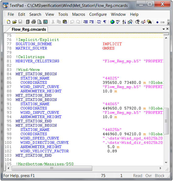
It is recommended to become familiar with the CMS-Flow Card File and view it using a text editor which allows syntax highlighting such as Textpad (see Figure 2 1) or Notepadd++ (see Figure 2 2). | It is recommended to become familiar with the CMS-Flow Card File and view it using a text editor which allows syntax highlighting such as Textpad (see Figure 2-1) or Notepadd++ (see Figure 2-2). | ||
[[File:fig_2-1.png]] | |||
Figure 2-1. CMS-FlowCard File viewed in TextPad. | |||
[[File:fig_2-1.png]] | |||
Figure 2-2. CMS-Flow Card File viewed in Notepad++. | |||
==Tips== | |||
:1. It is recommended to become familiar with the CMS-Flow card file and to learn how to manually edit and enter cards without having to use the SMS interface. When the user saves the CMS-Flow project in SMS, all of the input files are rewritten including the grid and model parameters file (which can be large). Therefore if only one parameter needs to be changed in the card file, it is much easier and faster to open the card file, manually edit the field, and re-save the card file instead of potentially having to reload the project in SMS, wait for the project to display, open the ''Model Control Window'', edit the input parameter, and re-save the project. | |||
:2. It is recommended to view the CMS-Flow Card File in a text editor which supported user-defined syntax highlighting such as Notepad++, Textpad, and UltraEdit. Syntax definitions for Textpad and Notepadd++ are available from the CIRP wiki website at http://cirp.usace.army.mil/wiki/Utilities. | |||
:3. Since all of the statements after the <span style="color:#0000FF">END_PARAMETERS</span> card are ignored. This section of the card file is useful for placing metadata or cards saving card sections when testing different model setups. | |||
:4. There are basically two types of cards in CMS: (1) single line cards, and (2) block declaration cards. Single line cards have input arguments specified on the same line as the card and in general to not depend on the order in which the cards are specified. Block declaration cards specify the beginning and end of a block. Blocks are used to group several input parameter statements. Blocks may contain multiple single line cards or other blocks. | |||
==Output Files== | |||
The minimum output files are the ''XMDF Global Solution File'' (*.h5), the Diagnostic File (CMS_DIAG.txt). By default, all of the solution variables are output to the same Global Solution File, but it is possible If ''Observation Cells (Save Points)'' are selected for output time series at individual cells, then additional ASCII files are written for each of the output varia-bles. More information on the ''Observation Cells'' is provided in the section <span style="color:#0000FF">Output: Observation Cells (Save Points)</span>. | |||
Table 2-12. CMS-Flow Output Files | |||
{|class="wikitable" | |||
|- | |||
!File | |||
!Name | |||
!Description | |||
|- | |||
|XMDF Global Solution Files | |||
|*_sol.h5 | |||
*_wse.h5 | |||
*_vel.h5 | |||
*_visc.h5 | |||
*_wave.h5 | |||
*_morph.h5 | |||
*_trans.h5 | |||
|XMDF file containing the time varying global solution including water levels, current velocities, etc. The different files are described in detail in the Output section of this document. | |||
|- | |||
|Diagnostic File | |||
|CMS_DIAG.txt | |||
|Name of the CMS-Flow Diagnostic File. Contains the model setup, time stepping history, subset of the screen output. | |||
|- | |||
|Observation Cells (Save Point) Files | |||
|*.txt | |||
|Specifies the coordinates, and depths of the CMS-Flow grid(s). If a telescoping grid is used, multiple grids are saved for each refinement level. | |||
|- | |||
|Super ASCII Global Solution Files | |||
|*.sup | |||
*.xy | |||
*.dat | |||
|SMS ASCII file containing the time varying global solution including water levels, current velocities, etc. | |||
|- | |||
|Tecplot ASCII Global Solution Files | |||
|*.dat | |||
*.his | |||
|Tecplot ASCII file containing the time varying global solution including water levels, current velocities, etc. | |||
|} | |||
==Overview of SMS Interface== | |||
All of the CMS-Flow model parameters, settings, and output options are controlled from the ''CMS-Flow Model Control Window'' (see Figure below). The window also has a section for Advanced Cards in which features and options can be entered which have not been incorporated into the SMS interface yet or more advanced model features more experienced users. | |||
[[File:fig_2-3.png]] | |||
Figure 2 3. CMS-Flow Model Control: Model Parameters tab for specifying time series output of CMS-Flow calculated datasets. | |||
[[File:fig_2-4.png]] | |||
Figure 2 4. General Tab of th CMS-Flow Model Control window in SMS 11.1. | |||
==Geospatial Information== | |||
===Horizontal Coordinate Systems and Conventions=== | |||
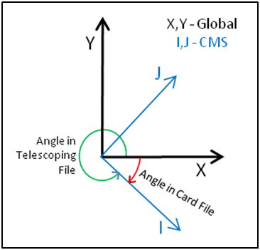
CMS-Flow uses a local coordinate system in which all vector values are positive along the I and J axis (Figure 4-2). All output vector arrays are specified in the local coordinate system. Any input that is specified on the local grid must be specified in the local coordinate system (e.g. initial condition for currents, interpolated wave forcing, etc). If input vector arrays are specified on a different grid, such as a spatially variable wind field or waves on a CMS-Wave grid, then the vectors are assumed to follow the coordinate system of their native grid. The grid is always created in SMS with the origin is by default always at the lower left hand corner of the grid. | CMS-Flow uses a local coordinate system in which all vector values are positive along the I and J axis (Figure 4-2). All output vector arrays are specified in the local coordinate system. Any input that is specified on the local grid must be specified in the local coordinate system (e.g. initial condition for currents, interpolated wave forcing, etc). If input vector arrays are specified on a different grid, such as a spatially variable wind field or waves on a CMS-Wave grid, then the vectors are assumed to follow the coordinate system of their native grid. The grid is always created in SMS with the origin is by default always at the lower left hand corner of the grid. | ||
[[File:fig_2-5.png]] | |||
Figure 2-5. CMS-Flow local coordinate system and grid angle conventions used in the Card and Telescoping Grid Files. The I and J axis indicate the CMS grid axis, while the X and Y axis indicate the global coordinate system. | |||
In the SMS, the term “projection” refers to a horizontal map projection such as “State Plane” or “Geographic”. Within the software, a global pro-jection can be associated with a project. Individual datasets may also have their own projections, which if properly associated with their original reference, can be displayed without the global projection reference. Previous versions of the SMS software referred to projections as “coordinate systems” and reprojection as “coordinate conversion”. | In the SMS, the term “projection” refers to a horizontal map projection such as “State Plane” or “Geographic”. Within the software, a global pro-jection can be associated with a project. Individual datasets may also have their own projections, which if properly associated with their original reference, can be displayed without the global projection reference. Previous versions of the SMS software referred to projections as “coordinate systems” and reprojection as “coordinate conversion”. | ||
The projection for the project can be specified from the Edit | Projection pull-down menu command. Changing the projection does not alter the coordinates of the project data. To change the projection of the individual project data, the dataset must be reprojected to the common reference system. The CMS models operate in a Cartesian coordinate system such as State Plane or UTM. | |||
The projection for the project can be specified from the ''Edit | Projection'' pull-down menu command. Changing the projection does not alter the coordinates of the project data. To change the projection of the individual project data, the dataset must be reprojected to the common reference system. The CMS models operate in a Cartesian coordinate system such as State Plane or UTM. | |||
Currently in SMS 11.1 the horizontal projection information in the grid file (*_grid.h5). The projection of the CMS-Flow simulation may be different from that of the grid and is specified in the CMS-Flow Control File. Specifying the projection information in the Control File is only necessary if any model input (such as wind or parent grids) is specified in any other projections. Otherwise the CMS assumes that all the horizontal projections are the same and no internal conversions are necessary. The table below describes the CMS-Flow cards used to specify the horizontal projection. | Currently in SMS 11.1 the horizontal projection information in the grid file (*_grid.h5). The projection of the CMS-Flow simulation may be different from that of the grid and is specified in the CMS-Flow Control File. Specifying the projection information in the Control File is only necessary if any model input (such as wind or parent grids) is specified in any other projections. Otherwise the CMS assumes that all the horizontal projections are the same and no internal conversions are necessary. The table below describes the CMS-Flow cards used to specify the horizontal projection. | ||
Table 2-13. CMS-Flow cards related to the single tidal water level boundary condition. | |||
{|class="wikitable" | |||
|- | |||
Input | |||
Card Format | |||
Notes | |||
|- | |||
|Start of | |||
Horizontal | |||
Projection | |||
Block | |||
|[begin=(HORIZONTAL_PROJECTION_BEGIN, | |||
HORIZ_PROJ_BEGIN), | |||
version=4.0, block=HorizProj, | |||
children=(HorizDatum,HorizCoord, | |||
HorizZone,HorizUnits)] | |||
|Begins the block structure for specifying the horizontal projection. | |||
|- | |||
|Horizontal | |||
Datum | |||
|[card=DATUM, parent=HorizProj] | |||
[arg=HorizDatum, type=char, | |||
options=(NAD27,NAD83,LOCAL), | |||
default= LOCAL] | |||
|Specifies the horizontal datum. | |||
|- | |||
|Horizontal | |||
Coordinate | |||
System | |||
|[card=SYSTEM] | |||
[arg=HorizCoord, type=char, | |||
options=(STATE_PLANE,UTM, | |||
GEOGRAPHIC,LOCAL), | |||
default=LOCAL, parent=HorizProj] | |||
|Specifies the horizontal coordinate system. | |||
|- | |||
|Horizontal | |||
Zone | |||
|[card=ZONE] | |||
[arg=HorizZone, type=int, | |||
default=none, parent=HorizProj] | | |||
|Specifies the horizontal zone (only valid for UTM and State Plane Coordinate Systems). | |||
|- | |||
|Horizontal | |||
Units | |||
|[card=UNITS] | |||
[arg=HorizUnits, type=char, | |||
options=(METERS,FEET,DEGREES, | |||
RADIANS), default=METERS, | |||
parent=HorizProj] | |||
|Specifies the units of the horizontal coordinate system. | |||
|- | |||
|End of | |||
Horizontal | |||
Projection | |||
Block | |||
|[end=(HORIZONTAL_PROJECTION_END, | |||
HORIZ_PROJ_END), | |||
version=4.0, block=HorizProj, | |||
childs=(HorizDatum,HorizCoord, | |||
HorizZone,HorizUnits)] | |||
|Ends the block structure for specifying the vertical projection. | |||
|} | |||
Example 2-2. Specifying the horizontal projection information. | |||
<span style="color:#8A2BE2">HORIZONTAL_PROJECTION_BEGIN</span> <span style="color:#008000">!can also use HORIZ_PROJ_BEGIN</span> | |||
<span style="color:#0000FF">DATUM</style> <span style="color:#008000">NAD83 !NAD27 | NAD83 | LOCAL</span> | |||
<span style="color:#0000FF">SYSTEM</span> <span style="color:#FF0000">STATE_PLANE</span> <span style="color:#008000">!UTM | STATE_PLANE | GEOGRAPHIC | LOCAL</span> | |||
<span style="color:#0000FF">UNITS</span> <span style="color:#FF0000">METERS</span> <span style="color:#008000">!METERS | FEET</span> | |||
<span style="color:#0000FF">ZONE</span> 3104 <span style="color:#008000">!Long Island, New York, Only if necessary</span> | |||
<span style="color:#8A2BE2">HORIZONTAL_PROJECTION_END</span> <span style="color:#008000">!can also use HORIZ_PROJ_END</span> | |||
A list of the supported horizontal datums, coordinate systems, or units are described in the following tables. | A list of the supported horizontal datums, coordinate systems, or units are described in the following tables. | ||
Table 2-14. Horizontal datums currently supported by CMS. | |||
{|class="wikitable" | |||
|- | |||
!Datum | |||
!Description | |||
|- | |||
|LOCAL | |||
|Local datum. Set as the default datum. May be used when a coordinate system is not defined or working with idealized cases. | |||
|- | |||
|NAD27 | |||
|Geographic coordinate system. | |||
|- | |||
|NAD83 | |||
|Universal Transverse Mercator (UTM) coordinate system. 2D Cartesian coordinate system. | |||
|} | |||
Table 2-15. Horizontal coordinate systems currently supported by CMS | |||
{|class="wikitable" | |||
|- | |||
!Coordinate | |||
Systems | |||
!Description | |||
|- | |||
|LOCAL | |||
|Local coordinate system. Set as the default coordinate system. May be used when a coordinate system is not defined or working with idealized cases. | |||
|- | |||
|UTM | |||
|Universal Transverse Mercator (UTM) coordinate system. 2D Cartesian coordinate system. | |||
|- | |||
|STATE_PLANE | |||
|State Plane coordinate system (also SPS or SPCS). Is divided into 124 geographic zones or coordinate systems designed for specific regions of the United States. Each State contains at least one zone. | |||
|- | |||
|GEOGRAPHIC | |||
|Geographic latitude and longitude coordinate system. | |||
|} | |||
Table 2-16. Horizontal coordinate units (HorizUnits) currently supported by CMS. | |||
{|class="wikitable" | |||
|- | |||
!Horizontal Units (HorizUnits) | |||
!Description | |||
|- | |||
|METERS | |||
|Units of meters only valid for State Plane and UTM coordinate system. | |||
|- | |||
|FEET | |||
|Units of feet only valid for State Plane and UTM coordinate system. | |||
|- | |||
|DEGREES | |||
|Units of degrees only valid for the Geographic coordinate system. | |||
|- | |||
|RADIANS | |||
|Units of radians only valid for the Geographic coordinate system. | |||
|- | |||
|SECONDS | |||
|Units of seconds only valid for the Geographic coordinate system. | |||
|} | |||
===Notes=== | |||
:In the CMS V4.1, it is not possible to convert between datums NAD27 and NAD83, therefore all of the input horizontal projections must have the same datum. | |||
In the CMS V4.1, it is not possible to convert between datums NAD27 and NAD83, therefore all of the input horizontal projections must have the same datum. | |||
Since the difference between the International Foot and US Survey Foot is 6.0960×10⁻⁷ m, the difference can be ignored for the purposes of coastal modeling and no differentiation is made between them in the CMS. | :Since the difference between the International Foot and US Survey Foot is 6.0960×10<sup>-7</sup> m, the difference can be ignored for the purposes of coastal modeling and no differentiation is made between them in the CMS. | ||
=Vertical Coordinate System and Conventions= | |||
Water depths in CMS are positive and land elevations are negative. The vertical reference Datum in CMS is a local datum. Therefore, any vertical datum can be used by the user. However, it is important to note that the default initial water surface elevation is set to zero with respect to the local datum. | Water depths in CMS are positive and land elevations are negative. The vertical reference Datum in CMS is a local datum. Therefore, any vertical datum can be used by the user. However, it is important to note that the default initial water surface elevation is set to zero with respect to the local datum. | ||
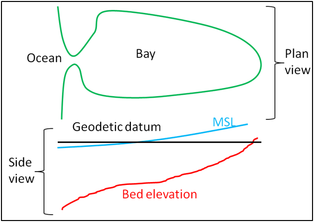
In choosing the vertical datum for CMS it is important to understand the differences between tidal and geodetic datums. It is common to use both types of datums. However, the most appropriate datum type depends on the project application. Tidal datums are a standard elevation defined by a tidal statistic such as the arithmetic mean of mean high water and mean low water over a tidal epoch known as the Mean Tide Level or MTL. Therefore, tidal datums vary spatially and in time. This is an important difference with respect to Geodetic datums such NAVD88 which are fixed reference elevations determined by geodetic leveling. Tidal datums should not be used for projects where the tidal datums vary spatially. It is common for bays to have tidal setup or super elevation of the mean water level caused by wind, fresh water inflow, and bottom friction. This will cause a difference in the MTL in the bay with respect to the ocean as illustrated in Figure 4-3. | In choosing the vertical datum for CMS it is important to understand the differences between tidal and geodetic datums. It is common to use both types of datums. However, the most appropriate datum type depends on the project application. Tidal datums are a standard elevation defined by a tidal statistic such as the arithmetic mean of mean high water and mean low water over a tidal epoch known as the Mean Tide Level or MTL. Therefore, tidal datums vary spatially and in time. This is an important difference with respect to Geodetic datums such NAVD88 which are fixed reference elevations determined by geodetic leveling. Tidal datums should not be used for projects where the tidal datums vary spatially. It is common for bays to have tidal setup or super elevation of the mean water level caused by wind, fresh water inflow, and bottom friction. This will cause a difference in the MTL in the bay with respect to the ocean as illustrated in Figure 4-3. | ||
[[File:fig_2-6.png]] | |||
Figure 2-6. Schematic of showing the difference between MSL (tidal) and geodetic datums. | |||
Currently, in CMS V4.1 the vertical projection information is only specified for metadata purposes and no internal conversions are performed yet. In the future, the goal is to be able to read in the vertical datum conversion conversions either from the model input files or to get them from an external database such as VDatum (http://vdatum.noaa.gov/welcome.html). A description of the cards used to specify the vertical projection is provided in the table below. | Currently, in CMS V4.1 the vertical projection information is only specified for metadata purposes and no internal conversions are performed yet. In the future, the goal is to be able to read in the vertical datum conversion conversions either from the model input files or to get them from an external database such as VDatum (http://vdatum.noaa.gov/welcome.html). A description of the cards used to specify the vertical projection is provided in the table below. | ||
Table 2-17. CMS-Flow cards related to the single tidal water level boundary condition. | |||
{|class="wikitable" | |||
|- | |||
!Card | |||
!Arguments | |||
!Description | |||
|- | |||
|Begin Vertical Projection Block | |||
|[begin=VERTICAL_PROJECTION_BEGIN, | |||
block=VertProj, version=4.0, | |||
childs=(VertDatum,VertUnits, | |||
VertOffset)] | |||
|Begins the block structure for specifying the vertical projection. | |||
|- | |||
|Vertical Datum | |||
|[card=DATUM, parent=VertProj] | |||
[name=VertDatum, type=char, | |||
options=(NGVD27,NAVD88,LOCAL, | |||
MSL,MTL,MLW,MLLW,MHW,MHHW), | |||
default=LOCAL] | |||
|Specifies the vertical datum. | |||
|- | |||
|Vertical Units | |||
|[card= UNITS, parent=VertProj] | |||
[name=VertUnits, type=char, | |||
options=(‘m’,‘ft’), | |||
default=‘m’] | |||
|Specifies the units of the vertical coordinate. | |||
|- | |||
|Vertical Offset | |||
|[card=OFFSET, comment=”positive | |||
is upwards”] | |||
[name=VertOffset, type=float, | |||
limits=none, parent=VertProj] | |||
|Specifies the vertical offset from the datum specified. | |||
Useful for referencing a local datum to a known vertical datum. Positive is upwards and negative is downwards. | |||
|- | |||
|Ends Vertical Projection Block | |||
|[end=VERTICAL_PROJECTION_END, | |||
block=VertProj,version=4.0, | |||
childs=(VertDatum,VertUnits, | |||
VertOffset)] | |||
|Ends the block structure for specifying the vertical projection. | |||
|} | |||
Example 2-3. Vertical projection specification. | |||
<span style="color:#8A2BE2">VERTICAL_PROJECTION_BEGIN</span> <span style="color:#008000">!Optional</span> | |||
<span style="color:#0000FF">DATUM</span> <span style="color:#FF0000">NAVD88</span> <span style="color:#008000">!NGVD29 | NAVD88 | LOCAL</span> | |||
<span style="color:#0000FF">UNITS</span> <span style="color:#FFA500">‘m'</span> <span style="color:#008000">!‘m’ | ‘ft’</span> | |||
<span style="color:#0000FF">OFFSET</span> 0.0 <span style="color:#FFA500">‘m’</span> <span style="color:#008000">!Positive is upwards</span> | |||
<span style="color:#8A2BE2">VERTICAL_PROJECTION_END</span> | |||
The vertical offset is useful for referencing a local datum to a known vertical datum as in the example above. In CMS, the default initial water level (can be specified otherwise using a hot start file) and therefore it is com-mon practice to use a vertical datum which is close to MSL. However, be-cause MSL is a tidal datum and therefore varies spatially, it is more accu-rate to use a geodetic datum with an offset, so that the zero reference elevation of the local datum is close to MSL. | The vertical offset is useful for referencing a local datum to a known vertical datum as in the example above. In CMS, the default initial water level (can be specified otherwise using a hot start file) and therefore it is com-mon practice to use a vertical datum which is close to MSL. However, be-cause MSL is a tidal datum and therefore varies spatially, it is more accu-rate to use a geodetic datum with an offset, so that the zero reference elevation of the local datum is close to MSL. | ||
Table 2-18. Horizontal datums currently supported by CMS. | |||
{|class="wikitable" | |||
|- | |||
!Datum | |||
!Description | |||
|- | |||
|LOCAL | |||
|Local datum. Set as the default datum. May be used when a coordinate system is not defined or working with idealized cases. | |||
|- | |||
|NGVD29 | |||
|National Geodetic Vertical Datum of 1929 | |||
|- | |||
|NAVD88 | |||
|National Geodetic Vertical Datum of 1988 | |||
|- | |||
|MSL | |||
|Mean Sea Level | |||
|- | |||
|MTL | |||
|Mean Tidal Level | |||
|- | |||
|MLW | |||
|Mean Low Water | |||
|- | |||
|MLLW | |||
|Mean Lower Low Water | |||
|- | |||
|MHW | |||
|Mean High Water | |||
|- | |||
|MHHW | |||
|Mean Higher High Water | |||
|} | |||
Notes: | Table 2-19. Horizontal coordinate units currently supported by CMS. | ||
1. If the project site is a small section of coastline with a small harbor or structures, then it is generally ok to use a tidal datum. | {|class="wikitable" | ||
2. If the project site includes an estuary, it is recommended to use a geodetic datum. | |- | ||
3. When using a geodetic datum in combination with tidal constituent forcing, it is recommended to offset the entire bathymetry so that the geodetic datum matches the offshore MSL. The reason for this is that tidal constituent | !Units | ||
boundary assumes that the reference datum is MSL. In CMS V4.1 it is possible to specify the MSL with respect to the CMS-Flow vertical datum. | !Description | ||
4. When using a geodetic datum in combination with water level time series, it is important to make sure the time series has the same geodetic datum as the bathymetry. In addition, an initial water level may be specified which is close to MSL (see the Hot Start section for details). | |- | ||
5. The units of the horizontal coordinate system should always be set to meters. By default, in SMS the horizontal units are set to feet. It is recommended to change the units to meters and save this setting by clicking on the menu File | Save Settings. This will save the horizontal projection and will be set every time SMS opens. | |METERS | ||
6. A good merged bathymetric dataset is often the result of spending 50% of the time it takes to get the model up and running just on checking and cleaning up the bathymetry alone. If a significant amount of time is spent paying attention to detail, there will be less instability problems in the hydrodynamic model which are difficult to trace back to the source. | |Units of meters only valid for State Plane and UTM coordinate system. | ||
7. Always double check that you have calculated your datum corrections very carefully by analyzing and comparing to nearby datasets. | |- | ||
8. When merging bathymetry, try both methods to combine the datasets and evaluate for depth consistency and dataset coverage. | |FEET | ||
9. Save often, and occasionally save new versions of your merge-testing in new folders. If you delete too much of one dataset, its useful to have the older, datum converted and unaltered datasets. | |Units of feet only valid for State Plane and UTM coordinate system. | ||
|} | |||
==Notes== | |||
:1. If the project site is a small section of coastline with a small harbor or structures, then it is generally ok to use a tidal datum. | |||
:2. If the project site includes an estuary, it is recommended to use a geodetic datum. | |||
:3. When using a geodetic datum in combination with tidal constituent forcing, it is recommended to offset the entire bathymetry so that the geodetic datum matches the offshore MSL. The reason for this is that tidal constituent boundary assumes that the reference datum is MSL. In CMS V4.1 it is possible to specify the MSL with respect to the CMS-Flow vertical datum. | |||
:4. When using a geodetic datum in combination with water level time series, it is important to make sure the time series has the same geodetic datum as the bathymetry. In addition, an initial water level may be specified which is close to MSL (see the Hot Start section for details). | |||
:5. The units of the horizontal coordinate system should always be set to meters. By default, in SMS the horizontal units are set to feet. It is recommended to change the units to meters and save this setting by clicking on the menu ''File | Save Settings''. This will save the horizontal projection and will be set every time SMS opens. | |||
:6. A good merged bathymetric dataset is often the result of spending 50% of the time it takes to get the model up and running just on checking and cleaning up the bathymetry alone. If a significant amount of time is spent paying attention to detail, there will be less instability problems in the hydrodynamic model which are difficult to trace back to the source. | |||
:7. Always double check that you have calculated your datum corrections very carefully by analyzing and comparing to nearby datasets. | |||
:8. When merging bathymetry, try both methods to combine the datasets and evaluate for depth consistency and dataset coverage. | |||
:9. Save often, and occasionally save new versions of your merge-testing in new folders. If you delete too much of one dataset, its useful to have the older, datum converted and unaltered datasets. | |||
==Cartesian Grids== | |||
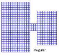
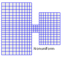
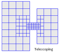
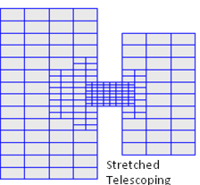
SMS supports regular and nonuniform Cartesian grids as well as regular and stretched telescoping grids (see Figure 4-4). | SMS supports regular and nonuniform Cartesian grids as well as regular and stretched telescoping grids (see Figure 4-4). | ||
[[File:fig_2-7aa.png|200px]][[File:fig_2-7bb.png|200px]] | |||
[[File:fig_2-7cc.png|200px]][[File:fig_2-7dd.png|200px]] | |||
Figure 2-7. Types of Cartesian grids supported by the SMS interface and CMS-Flow. | |||
Regular Cartesian grids are the easiest to generate making them useful for feasibility type studies, simple field cases, or test runs for more complicated field cases. Nonuniform Cartesian grids allow local refinement by gradually varying the grid spacing. These grids are offer more flexibility than regular Cartesian grids for a relatively low additional cost in generation. Nonuniform Cartesian grids are available for both CMS-Flow and CMS-Wave. For large complex modeling domains, Telescoping grids offer the most flexibility by providing local refine through the subdivision or splitting of cells into four. In many cases, the hydrodynamics can be aligned with one of the Cartesian coordinates. For these cases, the number of grid cells can be reduced by using a stretched Telescoping grid. Currently in SMS, the stretched Telescoping grids can only have a constant aspect ratio between the grid resolution in the ''x'' and ''y'' directions. | |||
When a CMS-Flow project is saved, SMS writes an XMDF ''Grid File'' named “*_grid.h5”. If the grid is non-telescoping, this file contains the x and y coordinates as well as the water depths. If a telescoping grid is saved, then the SMS saves multiple-grids in the ''CMS-Flow XMDF Grid File'' which correspond to different levels of resolution of the telescoping grid. This information is only used by SMS. The information used in CMS when saving a telescoping grid is saved in the ''Telescoping Grid File'' with the extension “*.tel”. The ''Telescoping Grid File'' contains the cell coordinates, resolution, connectivity and water depths. A description of ''XMDF Grid File'' and the Telescoping Grid File along with Matlab scripts for reading these files are provided in <span style="color:#0000FF">Grid File (*_grid.h5) and ''Telescoping Grid File'' (*.tel) sections of Appendix A: Description of Input Files.</span> | |||
All Cartesian grids can be characterized by a grid angle (orientation), origin coordinates. These grid parameters are saved to the Card File. The table below provides a description of the CMS-Flow cards used to specify the grid information in CMS. | All Cartesian grids can be characterized by a grid angle (orientation), origin coordinates. These grid parameters are saved to the Card File. The table below provides a description of the CMS-Flow cards used to specify the grid information in CMS. | ||
Table 2-20. CMS-Flow cards related to the grid files and datasets. | |||
{|class="wikitable" | |||
|- | |||
!Input | |||
!Format | |||
!Notes | |||
|- | |||
|XMDF Grid File | |||
|[card=GRID_FILE] | |||
[name=GridFile, type=char, | |||
default=”CaseName_grid.h5”] | |||
|Specifies the XMDF grid file | |||
|- | |||
|Telescoping Grid File | |||
|[card= TELESCOPING, | |||
CMS_version=4.0, SMS_version=11.0] | |||
[name=TelFile, type=char, | |||
default=”CaseName.tel”] | |||
|Specifies the telescoping grid file name. | |||
|- | |||
|Bathymetric Dataset | |||
|[card=BATHYMETRIC_DATASET] | |||
[name=BathyFile, type=char, | |||
default=GridFile] | |||
[name=BathyPath, type=char, | |||
default=”CaseName/Datasets/Depth”] | |||
|Specifies the bathymetric dataset file and path. | |||
|- | |||
|Grid Angle or Orientation | |||
|[card=GRID_ANGLE] | |||
[name=GridAngle, type=float] | |||
[name=GridAngleUnits, type=char, | |||
default=’deg’] | |||
|Specifies the grid angle measured counter-clockwise from the East direction to the grid i-axis (x-axis). | |||
|- | |||
|Grid Origin | |||
(x-coordinate) | |||
|[card=GRID_ORIGIN_X] | |||
[name=GridOriginX, type=float] | |||
[name= GridOriginUnits, type=char, | |||
default=’m’] | |||
|Specifies the x-coordinate for the Cartesian grid | |||
|- | |||
|Grid Origin | |||
(y-coordinate) | |||
|[card=GRID_ORIGIN_Y] | |||
[name=GridOriginY, type=float] | |||
[name=GridOriginUnits, type=char, | |||
default=’m’] | |||
|Specifies the y-coordinate for the Cartesian grid | |||
|- | |||
|Cell Center Latitudes | |||
|[card=CELL_LATITUDES] | |||
[name=LatFile, type=char, | |||
default=MPfile] | |||
[name=LatPath, type=char, | |||
default=”CaseName/Datasets/Depth”] | |||
|Specifies the latitudes at the cell centers. | |||
|- | |||
|Average Latitude [card=AVERAGE_LATITUDE] | |||
[name=AvgLat, type=float] | |||
[name=AvgLatUnits, type=char, | |||
default=’deg’] | |||
|Specifies the average latitude for the grid which is used for the Coriolis parameter. | |||
|} | |||
The example below shows the Cartesian grid parameters defined in the CMS-Flow Model Control File. | The example below shows the Cartesian grid parameters defined in the CMS-Flow Model Control File. | ||
Example 2-4. Grid geometry specification. | |||
---- | |||
---- | |||
!Grid Geometry | |||
BATHYMETRY_DATASET "Flow_Shark_grid.h5" "Flow_Shark/Datasets/Depth" | |||
GRID_ANGLE 13.0 deg !Clock-wise from X-axes | |||
GRID_ORIGIN_X 186102.986504 m | |||
GRID_ORIGIN_Y 145761.404499 m | |||
CELL_LATITUDES "Flow_Shark_mp.h5" "PROPERTIES/Model Params/Lats" | |||
---- | |||
---- | |||
If specified and average latitude is calculated for the grid and used to estimate the Coriolis parameter. By default the cell latitudes are stored in the XMDF Model Parameters File. For additional details on this file see XMDF CMS-Flow Model Parameters File (*_mp.h5). | If specified and average latitude is calculated for the grid and used to estimate the Coriolis parameter. By default the cell latitudes are stored in the XMDF Model Parameters File. For additional details on this file see XMDF CMS-Flow Model Parameters File (*_mp.h5). | ||
Notes: | |||
1. The grid angle specified in the Card File and the Telescoping Grid File use different conventions (unfortunately). The angle in the Card file is measured counter-clockwise from the East direction to the grid x-axis, while the angle in the Telescoping Grid File is measured clock-wise also from the East direction to the grid x-axis. | ===Notes=== | ||
2. By default the XMDF Grid File also contains the bathymetry and other spatial datasets including the bottom friction, hard bottom, D50, etc. However, these datasets can be specified in separate files. | |||
3. If a telescoping grid is used, the bathymetry is included by default in both the XMDF Grid File and the Telescoping Grid File. However, the depths in the in Telescoping Grid have -999 values for inactive cells. These cells are internally removed from the computational grid. Therefore, when using telescoping grids, only the depth values in the Telescoping Grid File are used by CMS. | :1. The grid angle specified in the ''Card File'' and the ''Telescoping Grid File'' use different conventions (unfortunately). The angle in the Card file is measured counter-clockwise from the East direction to the grid x-axis, while the angle in the ''Telescoping Grid File'' is measured clock-wise also from the East direction to the grid x-axis. | ||
:2. By default the ''XMDF Grid File'' also contains the bathymetry and other spatial datasets including the bottom friction, hard bottom, D50, etc. However, these datasets can be specified in separate files. | |||
:3. If a telescoping grid is used, the bathymetry is included by default in both the ''XMDF Grid File'' and the ''Telescoping Grid File''. However, the depths in the in Telescoping Grid have -999 values for inactive cells. These cells are internally removed from the computational grid. Therefore, when using telescoping grids, only the depth values in the ''Telescoping Grid File'' are used by CMS. | |||
The SMS Cartesian Grid Module has several tools for creating and editing Cartesian grids. A brief description of the tools is provided below | The SMS Cartesian Grid Module has several tools for creating and editing Cartesian grids. A brief description of the tools is provided below | ||
Create 2D Grid Frame | ==[[File:50-1.png]]Create 2D Grid Frame== | ||
The 2D Cartesian Grid Frame (purple box) creation tool allows the user to visually specify the location and orientation of the grid in space. To create a grid frame, simple click three times to the desired length and width dimensions. SMS will complete the rectangle. | The 2D Cartesian Grid Frame (purple box) creation tool allows the user to visually specify the location and orientation of the grid in space. To create a grid frame, simple click three times to the desired length and width dimensions. SMS will complete the rectangle. | ||
==[[File:50-2.png]]Select 2D Grid Frame== | |||
A 2D Cartesian Grid Frame can be modified with this selection tool. Once the frame is generated, the edges can be modified, the grid can be rotated (by selecting a small circle usually found in the lower left part of the grid), and the grid can be selected (middle black square) for manipulating location or opening the Grid Properties dialog box. | A 2D Cartesian Grid Frame can be modified with this selection tool. Once the frame is generated, the edges can be modified, the grid can be rotated (by selecting a small circle usually found in the lower left part of the grid), and the grid can be selected (middle black square) for manipulating location or opening the Grid Properties dialog box. | ||
Select Row/ Select Column | ==[[File:50-3.png]]Select Cell== | ||
The Select Row and Select Column tools are used to select cell rows and col-umns, respectively. Multiple rows and columns are selected in the same manner as selecting multiple individual cells: holding the SHIFT key, etc. | |||
The ''Select Cell'' tool is used to select a grid cell. A single cell is selected by clicking on it. A second cell can be added to the selection list by holding the SHIFT key while selecting it. Multiple cells can be selected at once by dragging a box around them. A selected cell can be de-selected by holding the SHIFT key as it is clicked. When a single cell is selected, its Z coordi-nate is shown in the Edit Window. The Z coordinate can be changed by typing a new value in the edit field, which updates the depth function. If multiple cells are selected, the Z coordinate field in the Edit Window shows the average depth of all selected cells. If this value is changed, the new value will be assigned to all selected cells. With one cell selected, the Edit Window shows the cells ''i,j'' location. With multiple cells selected, the Edit Window shows the number of selected cells. | |||
When the Insert Column or Insert Row tools are active, clicking within a cell splits the row/column containing the selected cell, creating a new row or column in the grid. The Z-values of all split cells are the same as the original cells’ values. | |||
==[[File:50-4.png]]Select Row/[[File:50-5.png]] Select Column== | |||
The ''Select Row'' and ''Select Column'' tools are used to select cell rows and col-umns, respectively. Multiple rows and columns are selected in the same manner as selecting multiple individual cells: holding the SHIFT key, etc. | |||
==[[File:50-6.png]]Insert Column/[[File:50-7.png]] Insert Row== | |||
When the ''Insert Column'' or ''Insert Row'' tools are active, clicking within a cell splits the row/column containing the selected cell, creating a new row or column in the grid. The Z-values of all split cells are the same as the original cells’ values. | |||
==[[File:51-1.png]]Drag Column/ [[File:51-2.png]] Drag Row Boundary== | |||
The position of the edge of rows or columns in a grid can be changed with the ''Drag Column'' or ''Drag Row'' tools. These tools make one column/row narrower while making its neighbor wider. These tools allow for manual specification of the resolution in specific portions of the grid. Note that depth values are not adjusted, so significant dragging of boundaries should be avoided or depths should be re-interpolated after the boundaries are modified. | |||
==[[File:51-3.png]]Create Cell String== | |||
The ''Create Cell String'' tool allows the modeler to group a string of cells to-gether for the purpose of assigning boundary conditions. Cell strings are created automatically around water boundaries when a grid is generated. The user may create others as desired or delete and replace the automatically generated cell strings. When the ''Create Cell String'' tool is active, the modeler selects each cell to be added to the string. By holding down the SHIFT key, all boundary cells between the previously selected cell and the selected cell are added to the cell string. | |||
==[[File:51-4.png]]Select Cell String== | |||
To specify a boundary condition, the modeler must create a cell string along the desired boundary cells, and then select the cell string while the ''Select Cell String'' tool is active. Specification of a boundary condition for the selected cell string is conducted through the ''Assign BC'' dialog, which is accessed through the CMS-M2D pull-down menu. | |||
==Editing Spatial Datasets== | |||
Spatial datasets including the bottom roughness may be edited manually by selecting and modifying cells, using the ''Data Calculator'', or by interpolating from a scatter set. Figure 2 10 shows an example where the Manning's n coefficient was increased for Shark River Inlet to account for the presence of vertical piles. To manually edit a spatial dataset | |||
:1. Click on the Select Cell tool [[File:52-1.png]] in the Cartesian Grid module toolbar. | |||
:2. Select a single or multiple cells by either: | |||
2. Select a single or multiple cells by either: | |||
::a. Clicking on a single cell. | |||
[[File:fig_2-8c.png]] | |||
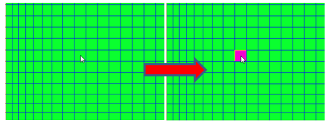
Figure 2-8. Selecting a single cell | |||
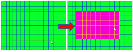
::b. Use a selection box by single-left-clicking and holding to drag a selection box over a group of cells. | |||
[[File:fig_2-9.png]] | |||
Figure 2-9. Selecting cell with a rectangle. | |||
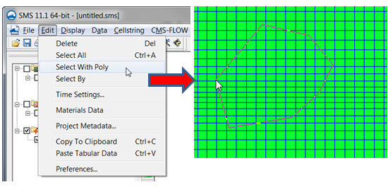
::c. Use a selection polygon by clicking on the menu ''Edit'' and selecting the submenu ''Select with Poly'' to select a group of cells with a polygon (see Figure below). | |||
[[File:fig_2-10.png]] | |||
Figure 2-10. Selecting cells with a polygon in SMS 11.1. | |||
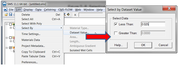
Figure 2 | ::d. Select cells by their value by clicking on the menu ''Edit'' and selecting the submenu ''Select By'' and then clicking the ''Data Set value…'' option (Figure 2-11). | ||
[[File:fig_2-11aa.png]] | |||
Figure 2-11. Selecting cells with a polygon in SMS. | |||
If the dataset being modified has been linked to a field such as the Man-ning’s n or the hard bottom in the CMS-Flow Control Window then the dataset will appear as editable in the SMS Edit Window (see Figure 2 12) and the user may proceed to Step 3. If the dataset does not appear as editable (i.e. the “S:” field is grayed-out), the dataset will need to temporarily set to the Elevation dataset in order to modify it. To set the dataset as the Elevation dataset follow the steps in Section <span style+"color:#0000FF">Mapping a Spatial Dataset as the Elevation Dataset</span>. | |||
:3. Enter a value in the “S:” field of the SMS Edit window (see Figure 2-12). | |||
[[File:fig_2-12.png|200px]] | |||
Figure 2-12. SMS Edit Window. | |||
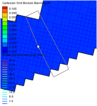
Figure 2-13 shows an example of a spatial dataset (Manning’s n in this case) which has manually been modified. | |||
[[File:fig_2-13.png]] | |||
Figure 2-13. Manning's ''n'' contours after modifying the areas under all three bridges. | |||
==Mapping a Spatial Dataset as the ''Elevation'' Dataset== | |||
The ''Elevation'' dataset is designated with the symbol [[File:55-1.png]] preceding the dataset name. As the name indicates, the ''Elevation'' dataset is elevation of the computational grid and is used within SMS for example when visualizing a grid in three dimensions. In CMS-Flow the ''Elevation'' dataset is typically called “Depth”. In some situations, it is useful to either temporarily designate a dataset as the Elevation dataset to be able to modify its values or to replace the ''Elevation'' dataset with a new one. To reset the ''Elevation'' dataset: | |||
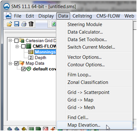
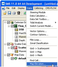
:1. Click on the menu ''Data | Map Elevation'' (Error! Reference source not found.). | |||
[[File:fig_2-14.png]] | |||
Figure 2-14. Selecting the Map Elevation menu option in SMS 11.1 | |||
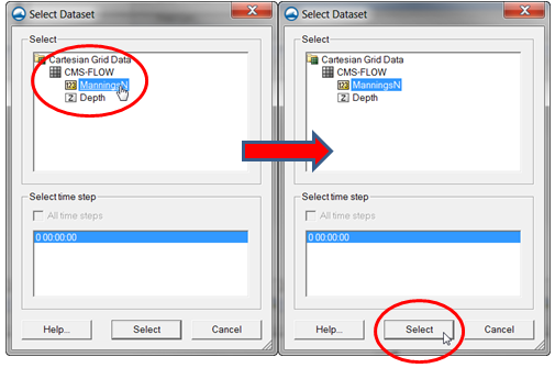
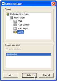
:2. In the SMS ''Select Dataset'' window, select the dataset to be converted as the Elevation dataset (Figure 2-15a) and then click on ''Select'' (Figure 2-15b). The select dataset friction dataset should now appear with the symbol [[File:55-1.png]] . | |||
[[File:fig_2-15.png]] | |||
Figure 2-15. Selecting the Map Elevation menu option in SMS 11.1 | |||
==Interpolating a Scatter Set to the Whole Grid== | |||
:1. Select the scatter set. | |||
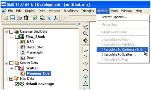
:2. Click on the menu Scatter | Interpolate to Cartesian Grid (see Figure 2-16). | |||
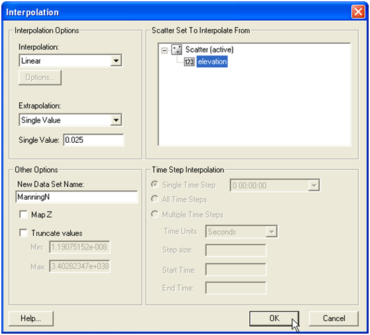
:3. In the Interpolation window, enter an extrapolation value, a name for the dataset and click OK (see Figure 2-17). | |||
[[File:fig_2-16.png]] | |||
Figure 2-16. Interpolating a scatter set of Manning's n values to the CMS-Flow grid. | |||
[[File:fig_2-17.png]] | |||
Figure 2-17. Interpolating a scatter set of Manning's n values to the CMS-Flow grid. | |||
The dataset will be interpolated to the whole grid and grid cells outside of the scatter triangulation will be set to the extrapolation value. | The dataset will be interpolated to the whole grid and grid cells outside of the scatter triangulation will be set to the extrapolation value. | ||
Interpolating a Scatter Set to a Portion of Grid | ==Interpolating a Scatter Set to a Portion of Grid== | ||
In some cases, it is desirable to only interpolate a bottom roughness scat-ter set to a portion of the grid. However, it is only possible to interpolate portions of the grid from scatters for the Elevation dataset. The Elevation dataset is the dataset with a | |||
In some cases, it is desirable to only interpolate a bottom roughness scat-ter set to a portion of the grid. However, it is only possible to interpolate portions of the grid from scatters for the Elevation dataset. The ''Elevation'' dataset is the dataset with a [[File:55-1.png]] to the left. Therefore, it is necessary to Map the bottom friction dataset as the ''Elevation'' dataset, interpolate the scatter set, and then re-map the actual grid elevation (usually named Depth) dataset as the ''Elevation'' dataset. The instructions for ''Mapping'' a dataset as the ''Elevation'' dataset is outlines in Section <span style="color:#0000FF">Mapping a Spatial Dataset as the Elevation Dataset</span>. To interpolate a bottom roughness dataset to a portion of a grid follow the instructions below. | |||
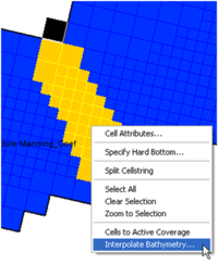
:1. Select the portion of the grid from which you want to interpolate the bottom friction dataset. This can be done by clicking and holding the left mouse button or by holding the Control key and single clicking so select the polygon and double clicking on the last polygon point (shown in Figure 2-18). | |||
:2. Once the correct cells are selected, right-click on the selected cells and select ''Interpolate Bathymetry''. | |||
[[File:fig_2-18a.png|200px]][[File:fig_2-18b.png|200px]] | |||
Figure 2 | Figure 2-18. Mapping of a dataset (bottom friction in this case) as the Elevation dataset. | ||
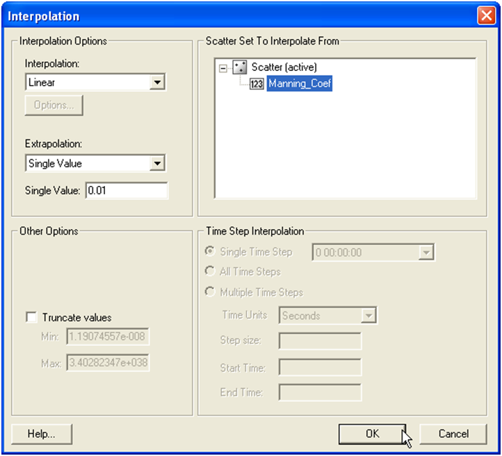
:3. In the interpolation window, select and appropriate extrapolation value and click ''OK'' (see Figure 2-19). | |||
[[File:fig_2-19.png]] | |||
Figure 2-19. SMS Interpolation window. | |||
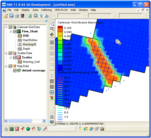
Figure 2-20 shows an example of how the final bottom friction dataset looks like once a portion of the dataset has been interpolated from a scatter set. | |||
[[File:fig_2-20.png]] | |||
Figure 2-20. SMS Interpolation window. | |||
:4. Re-map the ''Depth'' dataset as the Elevation dataset by clicking on Data | Map Elevation and selecting the Depth dataset (Figure 2-21). | |||
[[File:fig_2-21a.png|200px]][[File:fig_2-21b.png|200px]] | |||
Figure 2-21. Mapping of ''Depth'' dataset as the ''Elevation'' dataset. | |||
==Exporting a Dataset== | |||
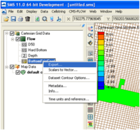
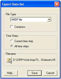
Exporting a spatially variable dataset such as bottom roughness (friction) datasets is useful for creating different project alternatives, scripting multiple runs, or for switching from different datasets for use as model input. Figure 2 22 illustrates how to export a dataset into an XMDF file. Multiple datasets can be exported into the same file. To export a dataset: | Exporting a spatially variable dataset such as bottom roughness (friction) datasets is useful for creating different project alternatives, scripting multiple runs, or for switching from different datasets for use as model input. Figure 2 22 illustrates how to export a dataset into an XMDF file. Multiple datasets can be exported into the same file. To export a dataset: | ||
1. Select the CMS-Flow dataset(s) in the SMS Project Explorer. | |||
2. Right-click and select the Export option. A window called Export Data Set will open | 1. Select the CMS-Flow dataset(s) in the ''SMS Project Explorer''. | ||
2. Right-click and select the ''Export'' option. A window called ''Export Data Set'' will open | |||
3. Under File Type select XMDF File. | 3. Under File Type select XMDF File. | ||
4. ''Under Time Steps'', select ''All time Steps'', even if the dataset only has one time step. | |||
5. Under ''Filename'' click on the folder icon and enter the location and filename for the dataset(s). | |||
[[File:fig_2-22a.png|200px]][[File:fig_2-22b.png|200px]] | |||
Figure 2-22. Manning’s ''n'' contours after modifying the areas under all three bridges. | |||
==CMS Input Format Version Number== | |||
An important aspect for all numerical models is version control. In CMS, the version of the input files is specifies in the first card in the CMS-Flow ''Card File''. A description of the card is provided in the table below. | |||
Table 2-21. Example input parameters and card formats | |||
{|class="wikitable" | |||
|- | |||
!Input | |||
!Format | |||
!Notes | |||
|- | |||
|CMS card file version | |||
|[card=CMS_VERSION] | |||
[name=version, type=float] | |||
|Specifies the version number of the CMS Card file. | |||
|} | |||
It is important to note that the version of the input files is separate from the CMS version number. CMS is designed to be backward compatible and as long as the input file version is equal to or lower than the CMS version, then the CMS will run properly. The version of the CMS executable is written to the CMS-Flow Diagnostic File (CMS_DIAG.txt). | It is important to note that the version of the input files is separate from the CMS version number. CMS is designed to be backward compatible and as long as the input file version is equal to or lower than the CMS version, then the CMS will run properly. The version of the CMS executable is written to the CMS-Flow Diagnostic File (CMS_DIAG.txt). | ||
Example 2-5. CMS Input format version number. | |||
---- | |||
---- | |||
<span style="color:#0000FF">CMS_VERSION<span> 4.0 <span style="color:#008000">!Version of input card file</span> | |||
---- | |||
---- | |||
==Timing== | |||
The starting time, time step, simulation duration, and ramp time are re-quired input parameters for CMS. A description of the cards used to specify the timing parameters is described in the table below. The starting time is input as a Julian date (year and day) and time (hour). | The starting time, time step, simulation duration, and ramp time are re-quired input parameters for CMS. A description of the cards used to specify the timing parameters is described in the table below. The starting time is input as a Julian date (year and day) and time (hour). | ||
The appropriate time step size is a function of the time stepping scheme (i.e. implicit or explicit), grid resolution, water depths, current velocities, and temporal variation of the solution. The explicit scheme time step is limited by the Courant-Friedrichs-Levy (CFL) condition | The appropriate time step size is a function of the time stepping scheme (i.e. implicit or explicit), grid resolution, water depths, current velocities, and temporal variation of the solution. The explicit scheme time step is limited by the Courant-Friedrichs-Levy (CFL) condition | ||
{{Equation|<math>C = \frac{\Delta t(|U| + \sqrt{gh})} {min(\Delta x,\Delta y)} \leq C_{max}</math>|2-1}} | |||
where | where <math>C_{max}</math> is the maximum Courant number typically set to 0.4-0.5. | ||
Since the implicit time stepping scheme is not limited by the CFL condi-tion for stability, a different criteria is needed. For coastal applications where tides are important, it is generally recommended to use at least 35-40 time steps for tidal wave period. For a semidiurnal tide with a period of 12 hrs, then the maximum time step is approximately 18 to 20 min. However if smaller tidal wave periods of 4 to 6 hrs are considered, then a maximum time step of approximately 9-10 minutes is reasonable. When using the implicit scheme, the time step is changed during the simulation if the model detects convergence problems. The time step is reduced by half until the convergence criteria have been met. Once the model detects that the time step can be increased, the time step is doubled. The initial time step is used as the maximum time step. | Since the implicit time stepping scheme is not limited by the CFL condi-tion for stability, a different criteria is needed. For coastal applications where tides are important, it is generally recommended to use at least 35-40 time steps for tidal wave period. For a semidiurnal tide with a period of 12 hrs, then the maximum time step is approximately 18 to 20 min. However if smaller tidal wave periods of 4 to 6 hrs are considered, then a maximum time step of approximately 9-10 minutes is reasonable. When using the implicit scheme, the time step is changed during the simulation if the model detects convergence problems. The time step is reduced by half until the convergence criteria have been met. Once the model detects that the time step can be increased, the time step is doubled. The initial time step is used as the maximum time step. | ||
The CMS does not interpolate global or point solutions in time, and therefore the initial time step should be chosen so that it is a multiple of the output intervals, or vice-versa, the output intervals should be chosen to be multiples of the initial step. | The CMS does not interpolate global or point solutions in time, and therefore the initial time step should be chosen so that it is a multiple of the output intervals, or vice-versa, the output intervals should be chosen to be multiples of the initial step. | ||
The simulation duration or length is specified in hours. The ramp period is the length of time during which the model forcing is gently increased or ramped from zero in order to avoid shocking the model at the beginning of the simulation. | The simulation duration or length is specified in hours. The ramp period is the length of time during which the model forcing is gently increased or ramped from zero in order to avoid shocking the model at the beginning of the simulation. | ||
Table 2-22. CMS-Flow Cards associated with timing. | |||
{|class="wikitable" | |||
|- | |||
!Input | |||
!Format | |||
!Notes | |||
|- | |||
|Simulation | |||
Starting | |||
Julian Day | |||
|[card=STARTING_JDATE] | |||
[name=StartJulDay, type=float, | |||
default=none] | |||
|Deprecated. Will be replaced in future releases with STARTING_DATE_TIME | |||
|- | |||
|Simulation | |||
Starting | |||
Hour | |||
|[card=STARTING_JDATE_HOUR] | |||
[name=StartJulDay, type=float, | |||
default=none] | |||
|Deprecated. Will be replaced in future releases with STARTING_DATE_TIME | |||
|- | |||
|Simulation Starting Date and Time | |||
|[card=STARTING_DATE_TIME] | |||
[name=StartDate0, type=char, | |||
default=none, example=”2004-12-24”] | |||
[name=StartTime0, type=char, | |||
default=none, example=”23:34:12”] | |||
[name=StartTimeZone, type=char, | |||
default=none, example=’UTC’ , | |||
otpional=true,] | |||
|Specifies the simulation starting calendar date and time. Double quotes are optional | |||
|- | |||
|Simulation | |||
Run | |||
Duration | |||
|[cards=(DURATION_RUN,SIMULATION_DURATION), | |||
CMS_versions=(4.0,4.1))]] | |||
[name=SimDur, type=float, | |||
default=none, limits=(SimDur>0.0)] | |||
[name=SimDurUnits, type=char, | |||
options=TimeUnits, default=’hrs’] | |||
|Sets the duration of the simulation in hours. | |||
|- | |||
|Ramp | |||
Duration | |||
|[cards=(DURATION_RAMP,RAMP_DURATION), | |||
CMS_versions=(4.0,4.1))] | |||
[name=RampDur, type=float, default=none, | |||
limits=(RampDur>0.0)] | |||
[name=RampDurUnits, type=char, | |||
options=TimeUnits, default=’hrs’] | |||
|Specifies the length of the ramp period. For details on the ramp period see the Ramp Period section. | |||
|} | |||
Example 2-6. General timing specification in CMS Versions 4.0 or earlier. | |||
---- | |||
---- | |||
!General timing cards | |||
STARTING_JDATE 80001 | |||
STARTING_JDATE_HOUR 0 | |||
DURATION_RUN 720.0 !hours | |||
DURATION_RAMP 1.0 !days | |||
---- | |||
---- | |||
Example 2-7. General timing specification in CMS Versions 4.1 and newer. | |||
---- | |||
---- | |||
!General timing cards | |||
STARTING_DATE_TIME 2004-12-24 23:34:12 UTC | |||
SIMULATION_DURATION 720.0 hrs !Units optional | |||
RAMP_DURATION 24.0 hrs | |||
---- | |||
---- | |||
==Tips== | |||
:1. The best way to determine the appropriate time step for an application is to conduct a sensitivity analysis. However, for most coastal applications an initial time step of 5-10 min is reasonable for the implicit scheme and a time step of 0.5-1.0 sec for the explicit scheme. | |||
example | :2. Use time steps that are multipliers of the output intervals. For example, it is common to output the hydrodynamics every 30 to 60 minutes, and so using a time step that is divisible by 30. | ||
==Notes== | |||
:1. The times in CMS-Flow are always referenced to Universal Time Coordinated (UTC). Prior to 1972, UTC was also called Greenwich Mean Time (GMT). | |||
1. The times in CMS-Flow are always referenced to Universal Time Coordinated (UTC). Prior to 1972, UTC was also called Greenwich Mean Time (GMT). | |||
Latest revision as of 14:11, 7 May 2015
2 CMS-Flow Model Setup
Overview of Input and Output
The CMS-Flow (and also for most morphodynamic models) input and output can be classified as:
- 1. Input
- a. Control file (model parameters, options, pointers to other files).
- b. Geometry (grid).
- c. Initial condition (bathymetry, bed composition, etc.).
- d. Boundary conditions
- 2. Output
- a. Transient solution
- i. Global (for the whole domain)
- ii. Point (at a single point or cell)
- b. Statistical parameters
- c. Hot start (may include internal variables)
- d. Diagnostic Files
A detailed description of the CMS input and output files is provided below.
Input Files
There are at least three required files to run CMS-Flow: (1) the Card File (*.cmcards), (2) the XMDF Grid File (*_grid.h5), (3) and the XMDF Model Parameters File. If a telescoping grid is used then an additional ASCII Telescoping Grid File is required. For a description of types of Cartesian grids available in CMS-Flow see section Cartesian Grids. If any input datasets such as the Manning’s coefficient or bed composition are specified in separate XMDF files then the file name and path must be specified in the Card File. Using separate input files for user-defined datasets makes it easier to make project alternatives or conduct sensitivity studies. The user-defined datasets can be easily created and exported from SMS. The procedure is described in detail in subsequent sections. A brief description of the CMS input files is provided in the table below.
Table 2-1. CMS-Flow Input Files
| File | Name | Description |
|---|---|---|
| Card File | *.cmcards | File name including path for the CMS-Wave sim file. |
| XMDF Grid File | *_grid.h5 | Specifies the coordinates, and depths of the CMS-Flow grid(s). If a telescoping grid is used, multiple grids are saved for each refinement level. |
| XMDF Model Parameters File | *_mp.h5 | Specifies boundary forcing information, wind forcing, and geographical coordinates. |
| Telescoping Grid File | *.tel | Specifies the cell coordinates, dimensions, and depths for the telescoping grid file. Only saved in the case a telescoping grid is used. |
| User-defined Dataset Files | *.h5 | Determines the extrapolation distance used for flow variables on the wave grid. |
CMS-Flow Card/Control File
In CMS-Flow, the Control File is an ASCII text file referred to also as the Card File because it contains a list of cards used to specify model input such as parameters, coefficients, options, etc. A card is simply a unique character string which the model uses to identify a specific model input. The Card File is the main input file which sets input parameters and points to other files. In general most of the “light” input data is specified in the Card File. Light data refers to input parameters which is relatively small in size and can easily be specified by the user in a few lines such as global parameters. Any input that is relatively large, such as time series, and spatially varying datasets are referred to as “heavy” data. Heavy data is stored in separate files such as the Grid File, Model Parameters File, or other user-specified files. The heavy data is then simply pointed to in the Card File.
Example 2-1. CMS-Flow Cards.
CMS_VERSION 4.0 !Version of input card file
BATHYMETRY_DATASET Flow_Shark_grid.h5" "Flow_Shark/Datasets/Depth"
GRID_ANGLE 13.0 ’deg’ !Clock-wise from X-axes
TIME_LIST_1 2 0.0 3.0 1.0 3.0 6.0 0.5
Formatting Rules and Conventions
The CMS-Flow Card File is a simple ASCII file with the following simple formatting rules and conventions:
- 1. Commented lines should be preceded by the characters ! or # or ignored. Comments can start at any column within the card file.
- 2. Cards are always written in capital letters.
- 3. Any character string in all capital letters after a card is an argument from a list options for that specific card (e.g. ON or OFF).
- 4. Card arguments are read in free-format. This means that input arguments should always be separated by at least one blank space or a comma.
- 5. Cards should always begin on a new line (i.e. only one card is allowed per line).
- 6. Character strings do not need to be enclosed in single or double quotation unless they contain white spaces. No characters besides letters (no accents) and numbers are allowed in character strings except: ‘(’, ‘)’, and ‘-’.
- 7. The end of the card file is specified by the END_PARAMETERS card. Any statements after this card are ignored.
Style Recommendations
The following recommendations are optional and provided for readability and to avoid commonly made formatting errors.
- 1. Single line cards should start at the first column unless the card is specified within a block in which case the card should be indented by 2 to 3 spaces.
- 2. Input arguments should start at column 37 for readability.
- 3. Double quotes should be used for file names and paths
- 4. Single quotes should be used for units.
Table 2-2. CMS-Flow Card notation.
| Notation | Description |
|---|---|
| ! | Indicates the beginning of a comment. Comments may begin at any column. Recommended for inserting headers and comments. |
| # | Indicates to ignore the rest of a line. Recommended for commenting cards. |
| ON | Activates a model feature |
| OFF | Deactivates a model feature |
| “ ” | Indicates a character string such as a file name or path |
| ‘ ’ | Indicates a character string for input argument units such as ‘m^3/s’ |
Many input cards have relationships to one another. For example a card may only be applicable if another card is specified. This is referred to here as a dependency. Dependencies are hierarchal in nature and may be listed either downwards or upwards in the dependency tree. One example of a dependency is the angle and repose and avalanching activation cards. The angle of repose is dependent on the avalanching being activated; otherwise it is not applicable. When two cards cannot exist together because they conflict with one another, this is referred to as an exclusion. An example of an exclusion is the bottom roughness specification using both a Manning’s n and bottom friction coefficient. The bottom roughness can only be specified once and therefore the input cards used to specify the Manning’s and bottom friction coefficient would conflict with one another. In the tables describing the input cards it is convenient to use to establish a notation for the card input formats.
Table 2-3. CMS-Flow Card format operators.
| Notation | Description |
|---|---|
| [] | Indicates a required input value (card or argument) |
| < | Specifies the range of an argument to be less than a value |
| > | Specifies the range of an argument to be greater than a value |
| <= | Specifies the range of an argument to be less or equal to a value |
| > | Specifies the range of an argument to be greater or equal to a value |
| = | Specifies the value(s) of an input argument |
Table 2-4. CMS-Flow Card Format key word description.
| Notation | Description |
|---|---|
| begin | Block structure begin statement |
| end | Block structure end statement |
| card | Character string for a card |
| arg | Variable name for a card argument |
| units | Unit type for input argument (generally optional) |
| options | List of card argument options |
| type | Argument type as floating (float), integer (int), or character (char) |
| float | Argument type as a real or floating |
| int | Argument type as an integer |
| char | Argument type as a character string |
| limits | Limits of the input argument if they exist |
| default | Argument default value if it exists. If an automatic default value is available then the automatic mode can be used. |
| dependencies | List of cards for which there exist a dependency |
| exclusions | List of cards for which there exist an exclusion |
| symbol | Mathematical symbol used for an input argument |
| required | Indicates whether in input argument is required or not |
| typical | Specifies a typical value or range for an input card. |
Below is an example of how the CMS-Flow cards are specified including com-ments at the end of each line.
Table 2-5. Example input parameters and card formats.
Input Format Notes| CMS card file version | [card=CMS_VERSION]
[name=version, type=float] |
Specifies the version number of the CMS Card file. |
| Implicit weighting factor | [card=IMPLICIT_WEIGHTING_FACTOR]
[arg=ImpWghtFac, symbol=θ, type=float, limits=(0.0<= ImpWghtFac<=1.0), default=0.0, required=false] |
ImpWghtFac =0 is first order and ImpWghtFac =1 is second order. |
| Sediment fall velocity value | [card=FALL_VELOCITY,
comment=’!units are optional’] [arg=SedFallVel, type=float, limits=(SedFallVel>0.0), required=false, default=automatic, dependencies=none, exclusions=FALL_VELOCITY_FORMULA] [units=SedFallVelUnits, type=char, options=VelocityUnits, default=‘m/s’] |
|
| Sediment fall velocity formula | [card= FALL_VELOCITY_FORMULA]
[arg=SedFallVelForm, type=char, options=(SOULSBY,WU), exclusions=FALL_VELOCITY] |
|
| Output time list | [card=( TIME_LIST_1, TIME_LIST_2,
TIME_LIST_3, TIME_LIST_4)] [type=int, name=nint, limits=(nint>=0)] for(i=1:nint,
[name=tstart(i), type=float,
limits=(tstart(i)>0.0)]
[name=tend(i), type=float,
limits=(tend(i)>=tstart(i))]
[name=tinc(i), type=float,
limits=(tinc(i)>=0.0)])
|
Table 2-6. Definition of Temperature Unit Character String Variables.
| TempUnits=(Celsius, Farhenheit, Kelvin, Rankin) |
| Celsius=(‘C’, ‘ºC’, ‘Celsius’) |
| Farhenheit=(‘F’, ‘ºF’, ‘Fahrenheit) |
| Kelvin=(‘K’, ‘ºK’, ‘Kelvin) |
| Rankin=(‘R’, ‘ºR’, ‘Rankin) |
Table 2-7. Definition of Angle Unit Character String Variables.
| AngleUnits=(Radians, Degrees) |
|---|
| Radians=(‘rad’, ‘radian’, ‘radians’ |
| Degrees=(‘deg’, ‘degree’, ‘degrees’, ‘º’) |
Table 2-8. Definition of Time Unit Character String Variables.
| TimeUnits=(Seconds, Minutes, Hours, Days, Weeks, Years) |
|---|
| Seconds=(‘s’, ‘sec’, ‘second’, ‘seconds’) |
| Minutes=(‘min’, ‘minute, ‘minutes’) |
| Hours=(‘h’, ‘hr’, ‘hrs’ ‘hour’, ‘hours’) |
| Days=(‘d’, ‘dy’, ‘day’, ‘days’) |
| Weeks=(‘w’, ‘wk’, ‘week’, ‘weeks’) |
| Years=(‘y’, ‘yr, ‘yrs’, ‘year’, ‘years’) |
Table 2-9. Definition of Length Unit Character String Variables.
| LengthUnits=(Micron, Millimeter, Centimeter, Kilometer, Inch, Feet) |
|---|
| Micron=(‘um’, ‘micron’, ‘microns’) |
| Millimeter=(‘mm’, ‘millimeter’, ‘millimeters’) |
| Centimeter=(‘cm’, ‘centimeter’, ‘centimeters’) |
| Meter =(‘m’, ‘meter’, ‘meters’) |
| Kilometer =(‘km’, ‘kilometer’, ‘kilometers’) |
| Inch =(‘in’, ‘inch’, ‘inches’) |
| Feet =(‘ft’, ‘foot’, ‘feet’) |
Table 2-10. Definition of Velocity Unit Character String Variables.
VelocityUnits=(mmps, cmps, mps, kph, fps, knot, mph)| mmps=(‘mmps’, ‘mm/s’, ‘mm/sec’, ‘millimeter/second’,
‘millimeters/second’) |
| cmps=(‘cmps’, ‘cm/s’, ‘cm/sec’, ‘centimeter/second’, ‘centimeters/second’) |
| mps=(‘mps’, ‘m/s’, ‘m/sec’, ‘meter/second’, ‘meter/second’) |
| kph=(‘kph’, ‘km/h’, ‘km/hr’, ‘kilometer/hour’, ‘kilometers/hour’) |
| fps=(‘fps’, ‘ftps’, ‘ft/s’, ‘ft/sec’, ‘feet/second’) |
| knots =(‘knot’, ‘knots’) |
| mph=(‘mph’, ‘mi/hr’, ‘miles/hour’) |
Table 2-11. Definition of Volume Flux Unit Character String Variables.
| VolumeFluxUnits=(cms, cmm, cmh, cfs, cfm, cfh, cmsc, cmmc, cmhc, cfsc, cfmc, cfhc) |
|---|
| cms=(‘cms’, ‘m^3/s’, ‘meter^3/sec’, ‘cubic meter/second’) |
| cmm=(‘cmm’, ‘m^3/min’, ‘meter^3/minute’, ‘cubic meter/minute’) |
| cmh=(‘cmh’, ‘m^3/hr’, ‘meter^3/hour’, ‘cubic meter/hour’) |
| cfs=(‘cfs’, ‘ft^3/s’, ‘ft^3/sec’, ‘cu ft/s’, ‘cubic foot/second’) |
| cfm=(‘cfm’, ‘ft^3/min’, ‘feet^3/minute’, ‘cu ft/s’, ‘cubic foot/minute’) |
| cfh=(‘cfh’, ‘ft^3/hr’, ‘ft^3/hour’, ‘cu ft/s’, ‘cubic foot/hour’) |
| cmsc=(‘cmsc’, ‘m^3/s/cell’, ‘meter^3/sec/cell’, ‘cubic meter/second/cell’) |
| cmmc=(‘cmmc’, ‘m^3/min/cell’, ‘meter^3/minute/cell’, ‘cubic meter/minute/cell’) |
| cmhc=(‘cmhc’, ‘m^3/hr/cell’, ‘meter^3/hour/cell’, ‘cubic meter/hour/cell’) |
| cfsc=(‘cfsc’, ‘ft^3/s/cell’, ‘ft^3/sec/cell’, ‘cu ft/s/cell’,‘cubic foot/second/cell’) |
| cfmc=(‘cfmc’, ‘ft^3/min/cell’, ‘feet^3/minute/cell’, ‘cu ft/s/cell’, ‘cubic foot/minute/cell’) |
| cfhc=(‘cfhc’, ‘ft^3/hr/cell’, ‘ft^3/hour/cell’, ‘cu ft/s/cell’, ‘cubic foot/hour/cell’) |
Note:
• The unit character strings are NOT case sensitive. Therefore, ‘km/hr’ is equivalent to ‘Km/hr’.
It is recommended to become familiar with the CMS-Flow Card File and view it using a text editor which allows syntax highlighting such as Textpad (see Figure 2-1) or Notepadd++ (see Figure 2-2).
Figure 2-1. CMS-FlowCard File viewed in TextPad.
Figure 2-2. CMS-Flow Card File viewed in Notepad++.
Tips
- 1. It is recommended to become familiar with the CMS-Flow card file and to learn how to manually edit and enter cards without having to use the SMS interface. When the user saves the CMS-Flow project in SMS, all of the input files are rewritten including the grid and model parameters file (which can be large). Therefore if only one parameter needs to be changed in the card file, it is much easier and faster to open the card file, manually edit the field, and re-save the card file instead of potentially having to reload the project in SMS, wait for the project to display, open the Model Control Window, edit the input parameter, and re-save the project.
- 2. It is recommended to view the CMS-Flow Card File in a text editor which supported user-defined syntax highlighting such as Notepad++, Textpad, and UltraEdit. Syntax definitions for Textpad and Notepadd++ are available from the CIRP wiki website at http://cirp.usace.army.mil/wiki/Utilities.
- 3. Since all of the statements after the END_PARAMETERS card are ignored. This section of the card file is useful for placing metadata or cards saving card sections when testing different model setups.
- 4. There are basically two types of cards in CMS: (1) single line cards, and (2) block declaration cards. Single line cards have input arguments specified on the same line as the card and in general to not depend on the order in which the cards are specified. Block declaration cards specify the beginning and end of a block. Blocks are used to group several input parameter statements. Blocks may contain multiple single line cards or other blocks.
Output Files
The minimum output files are the XMDF Global Solution File (*.h5), the Diagnostic File (CMS_DIAG.txt). By default, all of the solution variables are output to the same Global Solution File, but it is possible If Observation Cells (Save Points) are selected for output time series at individual cells, then additional ASCII files are written for each of the output varia-bles. More information on the Observation Cells is provided in the section Output: Observation Cells (Save Points).
Table 2-12. CMS-Flow Output Files
| File | Name | Description |
|---|---|---|
| XMDF Global Solution Files | *_sol.h5
|
XMDF file containing the time varying global solution including water levels, current velocities, etc. The different files are described in detail in the Output section of this document. |
| Diagnostic File | CMS_DIAG.txt | Name of the CMS-Flow Diagnostic File. Contains the model setup, time stepping history, subset of the screen output. |
| Observation Cells (Save Point) Files | *.txt | Specifies the coordinates, and depths of the CMS-Flow grid(s). If a telescoping grid is used, multiple grids are saved for each refinement level. |
| Super ASCII Global Solution Files | *.sup
|
SMS ASCII file containing the time varying global solution including water levels, current velocities, etc. |
| Tecplot ASCII Global Solution Files | *.dat
|
Tecplot ASCII file containing the time varying global solution including water levels, current velocities, etc. |
Overview of SMS Interface
All of the CMS-Flow model parameters, settings, and output options are controlled from the CMS-Flow Model Control Window (see Figure below). The window also has a section for Advanced Cards in which features and options can be entered which have not been incorporated into the SMS interface yet or more advanced model features more experienced users.
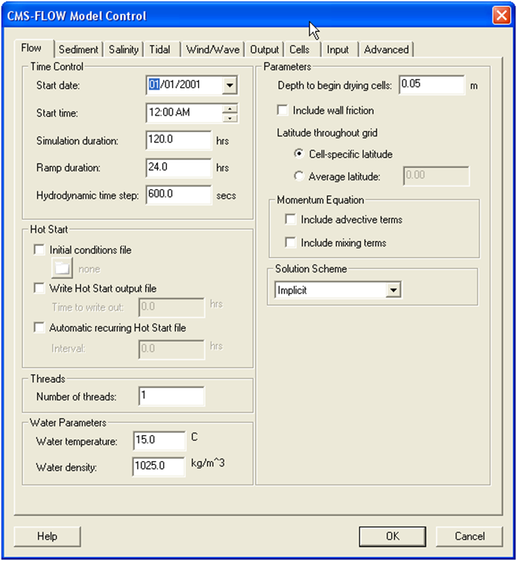 Figure 2 3. CMS-Flow Model Control: Model Parameters tab for specifying time series output of CMS-Flow calculated datasets.
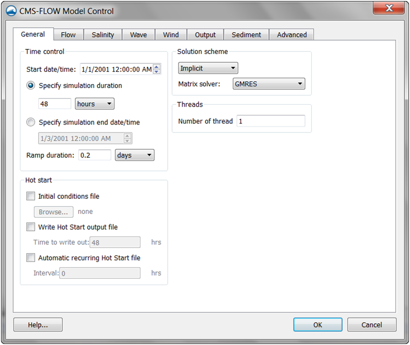 Figure 2 4. General Tab of th CMS-Flow Model Control window in SMS 11.1.
Geospatial Information
Horizontal Coordinate Systems and Conventions
CMS-Flow uses a local coordinate system in which all vector values are positive along the I and J axis (Figure 4-2). All output vector arrays are specified in the local coordinate system. Any input that is specified on the local grid must be specified in the local coordinate system (e.g. initial condition for currents, interpolated wave forcing, etc). If input vector arrays are specified on a different grid, such as a spatially variable wind field or waves on a CMS-Wave grid, then the vectors are assumed to follow the coordinate system of their native grid. The grid is always created in SMS with the origin is by default always at the lower left hand corner of the grid.
Figure 2-5. CMS-Flow local coordinate system and grid angle conventions used in the Card and Telescoping Grid Files. The I and J axis indicate the CMS grid axis, while the X and Y axis indicate the global coordinate system.
In the SMS, the term “projection” refers to a horizontal map projection such as “State Plane” or “Geographic”. Within the software, a global pro-jection can be associated with a project. Individual datasets may also have their own projections, which if properly associated with their original reference, can be displayed without the global projection reference. Previous versions of the SMS software referred to projections as “coordinate systems” and reprojection as “coordinate conversion”.
The projection for the project can be specified from the Edit | Projection pull-down menu command. Changing the projection does not alter the coordinates of the project data. To change the projection of the individual project data, the dataset must be reprojected to the common reference system. The CMS models operate in a Cartesian coordinate system such as State Plane or UTM.
Currently in SMS 11.1 the horizontal projection information in the grid file (*_grid.h5). The projection of the CMS-Flow simulation may be different from that of the grid and is specified in the CMS-Flow Control File. Specifying the projection information in the Control File is only necessary if any model input (such as wind or parent grids) is specified in any other projections. Otherwise the CMS assumes that all the horizontal projections are the same and no internal conversions are necessary. The table below describes the CMS-Flow cards used to specify the horizontal projection.
Table 2-13. CMS-Flow cards related to the single tidal water level boundary condition.
Input Card Format Notes| Start of
Horizontal Projection Block |
[begin=(HORIZONTAL_PROJECTION_BEGIN,
HORIZ_PROJ_BEGIN), version=4.0, block=HorizProj, children=(HorizDatum,HorizCoord, HorizZone,HorizUnits)] |
Begins the block structure for specifying the horizontal projection. |
| Horizontal
Datum |
[card=DATUM, parent=HorizProj]
[arg=HorizDatum, type=char, options=(NAD27,NAD83,LOCAL), default= LOCAL] |
Specifies the horizontal datum. |
| Horizontal
Coordinate System |
[card=SYSTEM]
[arg=HorizCoord, type=char, options=(STATE_PLANE,UTM, GEOGRAPHIC,LOCAL), default=LOCAL, parent=HorizProj] |
Specifies the horizontal coordinate system. |
| Horizontal
Zone |
[card=ZONE]
[arg=HorizZone, type=int, default=none, parent=HorizProj] | |
Specifies the horizontal zone (only valid for UTM and State Plane Coordinate Systems). |
| Horizontal
Units |
[card=UNITS]
[arg=HorizUnits, type=char, options=(METERS,FEET,DEGREES, RADIANS), default=METERS, parent=HorizProj] |
Specifies the units of the horizontal coordinate system. |
| End of
Horizontal Projection Block |
[end=(HORIZONTAL_PROJECTION_END,
HORIZ_PROJ_END), version=4.0, block=HorizProj, childs=(HorizDatum,HorizCoord, HorizZone,HorizUnits)] |
Ends the block structure for specifying the vertical projection. |
Example 2-2. Specifying the horizontal projection information.
HORIZONTAL_PROJECTION_BEGIN !can also use HORIZ_PROJ_BEGIN
  DATUM</style>           NAD83        !NAD27 | NAD83 | LOCAL
  SYSTEM          STATE_PLANE  !UTM | STATE_PLANE | GEOGRAPHIC | LOCAL
  UNITS           METERS       !METERS | FEET
  ZONE            3104         !Long Island, New York, Only if necessary
HORIZONTAL_PROJECTION_END !can also use HORIZ_PROJ_END
A list of the supported horizontal datums, coordinate systems, or units are described in the following tables.
Table 2-14. Horizontal datums currently supported by CMS.
| Datum | Description |
|---|---|
| LOCAL | Local datum. Set as the default datum. May be used when a coordinate system is not defined or working with idealized cases. |
| NAD27 | Geographic coordinate system. |
| NAD83 | Universal Transverse Mercator (UTM) coordinate system. 2D Cartesian coordinate system. |
Table 2-15. Horizontal coordinate systems currently supported by CMS
| Coordinate
Systems |
Description |
|---|---|
| LOCAL | Local coordinate system. Set as the default coordinate system. May be used when a coordinate system is not defined or working with idealized cases. |
| UTM | Universal Transverse Mercator (UTM) coordinate system. 2D Cartesian coordinate system. |
| STATE_PLANE | State Plane coordinate system (also SPS or SPCS). Is divided into 124 geographic zones or coordinate systems designed for specific regions of the United States. Each State contains at least one zone. |
| GEOGRAPHIC | Geographic latitude and longitude coordinate system. |
Table 2-16. Horizontal coordinate units (HorizUnits) currently supported by CMS.
| Horizontal Units (HorizUnits) | Description |
|---|---|
| METERS | Units of meters only valid for State Plane and UTM coordinate system. |
| FEET | Units of feet only valid for State Plane and UTM coordinate system. |
| DEGREES | Units of degrees only valid for the Geographic coordinate system. |
| RADIANS | Units of radians only valid for the Geographic coordinate system. |
| SECONDS | Units of seconds only valid for the Geographic coordinate system. |
Notes
- In the CMS V4.1, it is not possible to convert between datums NAD27 and NAD83, therefore all of the input horizontal projections must have the same datum.
- Since the difference between the International Foot and US Survey Foot is 6.0960×10⁻⁷ m, the difference can be ignored for the purposes of coastal modeling and no differentiation is made between them in the CMS.
Vertical Coordinate System and Conventions
Water depths in CMS are positive and land elevations are negative. The vertical reference Datum in CMS is a local datum. Therefore, any vertical datum can be used by the user. However, it is important to note that the default initial water surface elevation is set to zero with respect to the local datum.
In choosing the vertical datum for CMS it is important to understand the differences between tidal and geodetic datums. It is common to use both types of datums. However, the most appropriate datum type depends on the project application. Tidal datums are a standard elevation defined by a tidal statistic such as the arithmetic mean of mean high water and mean low water over a tidal epoch known as the Mean Tide Level or MTL. Therefore, tidal datums vary spatially and in time. This is an important difference with respect to Geodetic datums such NAVD88 which are fixed reference elevations determined by geodetic leveling. Tidal datums should not be used for projects where the tidal datums vary spatially. It is common for bays to have tidal setup or super elevation of the mean water level caused by wind, fresh water inflow, and bottom friction. This will cause a difference in the MTL in the bay with respect to the ocean as illustrated in Figure 4-3.
Figure 2-6. Schematic of showing the difference between MSL (tidal) and geodetic datums.
Currently, in CMS V4.1 the vertical projection information is only specified for metadata purposes and no internal conversions are performed yet. In the future, the goal is to be able to read in the vertical datum conversion conversions either from the model input files or to get them from an external database such as VDatum (http://vdatum.noaa.gov/welcome.html). A description of the cards used to specify the vertical projection is provided in the table below.
Table 2-17. CMS-Flow cards related to the single tidal water level boundary condition.
| Card | Arguments | Description |
|---|---|---|
| Begin Vertical Projection Block | [begin=VERTICAL_PROJECTION_BEGIN,
block=VertProj, version=4.0, childs=(VertDatum,VertUnits, VertOffset)] |
Begins the block structure for specifying the vertical projection. |
| Vertical Datum | [card=DATUM, parent=VertProj]
[name=VertDatum, type=char, options=(NGVD27,NAVD88,LOCAL, MSL,MTL,MLW,MLLW,MHW,MHHW), default=LOCAL] |
Specifies the vertical datum. |
| Vertical Units | [card= UNITS, parent=VertProj]
[name=VertUnits, type=char, options=(‘m’,‘ft’), default=‘m’] |
Specifies the units of the vertical coordinate. |
| Vertical Offset | [card=OFFSET, comment=”positive
is upwards”] [name=VertOffset, type=float, limits=none, parent=VertProj] |
Specifies the vertical offset from the datum specified.
Useful for referencing a local datum to a known vertical datum. Positive is upwards and negative is downwards. |
| Ends Vertical Projection Block | [end=VERTICAL_PROJECTION_END,
block=VertProj,version=4.0, childs=(VertDatum,VertUnits, VertOffset)] |
Ends the block structure for specifying the vertical projection. |
Example 2-3. Vertical projection specification.
VERTICAL_PROJECTION_BEGIN !Optional
 DATUM           NAVD88       !NGVD29 | NAVD88 | LOCAL
 UNITS           ‘m'       !‘m’ | ‘ft’
 OFFSET          0.0 ‘m’        !Positive is upwards
VERTICAL_PROJECTION_END
The vertical offset is useful for referencing a local datum to a known vertical datum as in the example above. In CMS, the default initial water level (can be specified otherwise using a hot start file) and therefore it is com-mon practice to use a vertical datum which is close to MSL. However, be-cause MSL is a tidal datum and therefore varies spatially, it is more accu-rate to use a geodetic datum with an offset, so that the zero reference elevation of the local datum is close to MSL.
Table 2-18. Horizontal datums currently supported by CMS.
| Datum | Description |
|---|---|
| LOCAL | Local datum. Set as the default datum. May be used when a coordinate system is not defined or working with idealized cases. |
| NGVD29 | National Geodetic Vertical Datum of 1929 |
| NAVD88 | National Geodetic Vertical Datum of 1988 |
| MSL | Mean Sea Level |
| MTL | Mean Tidal Level |
| MLW | Mean Low Water |
| MLLW | Mean Lower Low Water |
| MHW | Mean High Water |
| MHHW | Mean Higher High Water |
Table 2-19. Horizontal coordinate units currently supported by CMS.
| Units | Description |
|---|---|
| METERS | Units of meters only valid for State Plane and UTM coordinate system. |
| FEET | Units of feet only valid for State Plane and UTM coordinate system. |
Notes
- 1. If the project site is a small section of coastline with a small harbor or structures, then it is generally ok to use a tidal datum.
- 2. If the project site includes an estuary, it is recommended to use a geodetic datum.
- 3. When using a geodetic datum in combination with tidal constituent forcing, it is recommended to offset the entire bathymetry so that the geodetic datum matches the offshore MSL. The reason for this is that tidal constituent boundary assumes that the reference datum is MSL. In CMS V4.1 it is possible to specify the MSL with respect to the CMS-Flow vertical datum.
- 4. When using a geodetic datum in combination with water level time series, it is important to make sure the time series has the same geodetic datum as the bathymetry. In addition, an initial water level may be specified which is close to MSL (see the Hot Start section for details).
- 5. The units of the horizontal coordinate system should always be set to meters. By default, in SMS the horizontal units are set to feet. It is recommended to change the units to meters and save this setting by clicking on the menu File | Save Settings. This will save the horizontal projection and will be set every time SMS opens.
- 6. A good merged bathymetric dataset is often the result of spending 50% of the time it takes to get the model up and running just on checking and cleaning up the bathymetry alone. If a significant amount of time is spent paying attention to detail, there will be less instability problems in the hydrodynamic model which are difficult to trace back to the source.
- 7. Always double check that you have calculated your datum corrections very carefully by analyzing and comparing to nearby datasets.
- 8. When merging bathymetry, try both methods to combine the datasets and evaluate for depth consistency and dataset coverage.
- 9. Save often, and occasionally save new versions of your merge-testing in new folders. If you delete too much of one dataset, its useful to have the older, datum converted and unaltered datasets.
Cartesian Grids
SMS supports regular and nonuniform Cartesian grids as well as regular and stretched telescoping grids (see Figure 4-4).
Figure 2-7. Types of Cartesian grids supported by the SMS interface and CMS-Flow.
Regular Cartesian grids are the easiest to generate making them useful for feasibility type studies, simple field cases, or test runs for more complicated field cases. Nonuniform Cartesian grids allow local refinement by gradually varying the grid spacing. These grids are offer more flexibility than regular Cartesian grids for a relatively low additional cost in generation. Nonuniform Cartesian grids are available for both CMS-Flow and CMS-Wave. For large complex modeling domains, Telescoping grids offer the most flexibility by providing local refine through the subdivision or splitting of cells into four. In many cases, the hydrodynamics can be aligned with one of the Cartesian coordinates. For these cases, the number of grid cells can be reduced by using a stretched Telescoping grid. Currently in SMS, the stretched Telescoping grids can only have a constant aspect ratio between the grid resolution in the x and y directions.
When a CMS-Flow project is saved, SMS writes an XMDF Grid File named “*_grid.h5”. If the grid is non-telescoping, this file contains the x and y coordinates as well as the water depths. If a telescoping grid is saved, then the SMS saves multiple-grids in the CMS-Flow XMDF Grid File which correspond to different levels of resolution of the telescoping grid. This information is only used by SMS. The information used in CMS when saving a telescoping grid is saved in the Telescoping Grid File with the extension “*.tel”. The Telescoping Grid File contains the cell coordinates, resolution, connectivity and water depths. A description of XMDF Grid File and the Telescoping Grid File along with Matlab scripts for reading these files are provided in Grid File (*_grid.h5) and Telescoping Grid File (*.tel) sections of Appendix A: Description of Input Files.
All Cartesian grids can be characterized by a grid angle (orientation), origin coordinates. These grid parameters are saved to the Card File. The table below provides a description of the CMS-Flow cards used to specify the grid information in CMS.
Table 2-20. CMS-Flow cards related to the grid files and datasets.
| Input | Format | Notes |
|---|---|---|
| XMDF Grid File | [card=GRID_FILE]
[name=GridFile, type=char, default=”CaseName_grid.h5”] |
Specifies the XMDF grid file |
| Telescoping Grid File | [card= TELESCOPING,
CMS_version=4.0, SMS_version=11.0] [name=TelFile, type=char, default=”CaseName.tel”] |
Specifies the telescoping grid file name. |
| Bathymetric Dataset | [card=BATHYMETRIC_DATASET]
[name=BathyFile, type=char, default=GridFile] [name=BathyPath, type=char, default=”CaseName/Datasets/Depth”] |
Specifies the bathymetric dataset file and path. |
| Grid Angle or Orientation | [card=GRID_ANGLE]
[name=GridAngle, type=float] [name=GridAngleUnits, type=char, default=’deg’] |
Specifies the grid angle measured counter-clockwise from the East direction to the grid i-axis (x-axis). |
| Grid Origin
(x-coordinate) |
[card=GRID_ORIGIN_X]
[name=GridOriginX, type=float] [name= GridOriginUnits, type=char, default=’m’] |
Specifies the x-coordinate for the Cartesian grid |
| Grid Origin
(y-coordinate) |
[card=GRID_ORIGIN_Y]
[name=GridOriginY, type=float] [name=GridOriginUnits, type=char, default=’m’] |
Specifies the y-coordinate for the Cartesian grid |
| Cell Center Latitudes | [card=CELL_LATITUDES]
[name=LatFile, type=char, default=MPfile] [name=LatPath, type=char, default=”CaseName/Datasets/Depth”] |
Specifies the latitudes at the cell centers. |
| Average Latitude [card=AVERAGE_LATITUDE]
[name=AvgLat, type=float] [name=AvgLatUnits, type=char, default=’deg’] |
Specifies the average latitude for the grid which is used for the Coriolis parameter. |
The example below shows the Cartesian grid parameters defined in the CMS-Flow Model Control File.
Example 2-4. Grid geometry specification.
!Grid Geometry BATHYMETRY_DATASET "Flow_Shark_grid.h5" "Flow_Shark/Datasets/Depth" GRID_ANGLE 13.0 deg !Clock-wise from X-axes GRID_ORIGIN_X 186102.986504 m GRID_ORIGIN_Y 145761.404499 m CELL_LATITUDES "Flow_Shark_mp.h5" "PROPERTIES/Model Params/Lats"
If specified and average latitude is calculated for the grid and used to estimate the Coriolis parameter. By default the cell latitudes are stored in the XMDF Model Parameters File. For additional details on this file see XMDF CMS-Flow Model Parameters File (*_mp.h5).
Notes
- 1. The grid angle specified in the Card File and the Telescoping Grid File use different conventions (unfortunately). The angle in the Card file is measured counter-clockwise from the East direction to the grid x-axis, while the angle in the Telescoping Grid File is measured clock-wise also from the East direction to the grid x-axis.
- 2. By default the XMDF Grid File also contains the bathymetry and other spatial datasets including the bottom friction, hard bottom, D50, etc. However, these datasets can be specified in separate files.
- 3. If a telescoping grid is used, the bathymetry is included by default in both the XMDF Grid File and the Telescoping Grid File. However, the depths in the in Telescoping Grid have -999 values for inactive cells. These cells are internally removed from the computational grid. Therefore, when using telescoping grids, only the depth values in the Telescoping Grid File are used by CMS.
The SMS Cartesian Grid Module has several tools for creating and editing Cartesian grids. A brief description of the tools is provided below
 Create 2D Grid Frame
The 2D Cartesian Grid Frame (purple box) creation tool allows the user to visually specify the location and orientation of the grid in space. To create a grid frame, simple click three times to the desired length and width dimensions. SMS will complete the rectangle.
 Select 2D Grid Frame
A 2D Cartesian Grid Frame can be modified with this selection tool. Once the frame is generated, the edges can be modified, the grid can be rotated (by selecting a small circle usually found in the lower left part of the grid), and the grid can be selected (middle black square) for manipulating location or opening the Grid Properties dialog box.
 Select Cell
The Select Cell tool is used to select a grid cell. A single cell is selected by clicking on it. A second cell can be added to the selection list by holding the SHIFT key while selecting it. Multiple cells can be selected at once by dragging a box around them. A selected cell can be de-selected by holding the SHIFT key as it is clicked. When a single cell is selected, its Z coordi-nate is shown in the Edit Window. The Z coordinate can be changed by typing a new value in the edit field, which updates the depth function. If multiple cells are selected, the Z coordinate field in the Edit Window shows the average depth of all selected cells. If this value is changed, the new value will be assigned to all selected cells. With one cell selected, the Edit Window shows the cells i,j location. With multiple cells selected, the Edit Window shows the number of selected cells.
 Select Row/
 Select Column
The Select Row and Select Column tools are used to select cell rows and col-umns, respectively. Multiple rows and columns are selected in the same manner as selecting multiple individual cells: holding the SHIFT key, etc.
 Insert Column/
 Insert Row
When the Insert Column or Insert Row tools are active, clicking within a cell splits the row/column containing the selected cell, creating a new row or column in the grid. The Z-values of all split cells are the same as the original cells’ values.
 Drag Column/
  Drag Row Boundary
The position of the edge of rows or columns in a grid can be changed with the Drag Column or Drag Row tools. These tools make one column/row narrower while making its neighbor wider. These tools allow for manual specification of the resolution in specific portions of the grid. Note that depth values are not adjusted, so significant dragging of boundaries should be avoided or depths should be re-interpolated after the boundaries are modified.
 Create Cell String
The Create Cell String tool allows the modeler to group a string of cells to-gether for the purpose of assigning boundary conditions. Cell strings are created automatically around water boundaries when a grid is generated. The user may create others as desired or delete and replace the automatically generated cell strings. When the Create Cell String tool is active, the modeler selects each cell to be added to the string. By holding down the SHIFT key, all boundary cells between the previously selected cell and the selected cell are added to the cell string.
 Select Cell String
To specify a boundary condition, the modeler must create a cell string along the desired boundary cells, and then select the cell string while the Select Cell String tool is active. Specification of a boundary condition for the selected cell string is conducted through the Assign BC dialog, which is accessed through the CMS-M2D pull-down menu.
Editing Spatial Datasets
Spatial datasets including the bottom roughness may be edited manually by selecting and modifying cells, using the Data Calculator, or by interpolating from a scatter set. Figure 2 10 shows an example where the Manning's n coefficient was increased for Shark River Inlet to account for the presence of vertical piles. To manually edit a spatial dataset
- 2. Select a single or multiple cells by either:
- a. Clicking on a single cell.
Figure 2-8. Selecting a single cell
- b. Use a selection box by single-left-clicking and holding to drag a selection box over a group of cells.
Figure 2-9. Selecting cell with a rectangle.
- c. Use a selection polygon by clicking on the menu Edit and selecting the submenu Select with Poly to select a group of cells with a polygon (see Figure below).
Figure 2-10. Selecting cells with a polygon in SMS 11.1.
- d. Select cells by their value by clicking on the menu Edit and selecting the submenu Select By and then clicking the Data Set value… option (Figure 2-11).
Figure 2-11. Selecting cells with a polygon in SMS.
If the dataset being modified has been linked to a field such as the Man-ning’s n or the hard bottom in the CMS-Flow Control Window then the dataset will appear as editable in the SMS Edit Window (see Figure 2 12) and the user may proceed to Step 3. If the dataset does not appear as editable (i.e. the “S:” field is grayed-out), the dataset will need to temporarily set to the Elevation dataset in order to modify it. To set the dataset as the Elevation dataset follow the steps in Section Mapping a Spatial Dataset as the Elevation Dataset.
- 3. Enter a value in the “S:” field of the SMS Edit window (see Figure 2-12).
Figure 2-12. SMS Edit Window.
Figure 2-13 shows an example of a spatial dataset (Manning’s n in this case) which has manually been modified.
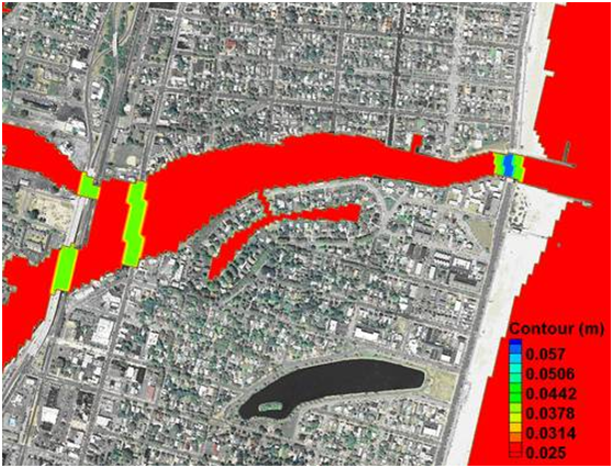 Figure 2-13. Manning's n contours after modifying the areas under all three bridges.
Mapping a Spatial Dataset as the Elevation Dataset
The Elevation dataset is designated with the symbol ![]() preceding the dataset name. As the name indicates, the Elevation dataset is elevation of the computational grid and is used within SMS for example when visualizing a grid in three dimensions. In CMS-Flow the Elevation dataset is typically called “Depth”. In some situations, it is useful to either temporarily designate a dataset as the Elevation dataset to be able to modify its values or to replace the Elevation dataset with a new one. To reset the Elevation dataset:
preceding the dataset name. As the name indicates, the Elevation dataset is elevation of the computational grid and is used within SMS for example when visualizing a grid in three dimensions. In CMS-Flow the Elevation dataset is typically called “Depth”. In some situations, it is useful to either temporarily designate a dataset as the Elevation dataset to be able to modify its values or to replace the Elevation dataset with a new one. To reset the Elevation dataset:
- 1. Click on the menu Data | Map Elevation (Error! Reference source not found.).
Figure 2-14. Selecting the Map Elevation menu option in SMS 11.1
- 2. In the SMS Select Dataset window, select the dataset to be converted as the Elevation dataset (Figure 2-15a) and then click on Select (Figure 2-15b). The select dataset friction dataset should now appear with the symbol
 .
.
Figure 2-15. Selecting the Map Elevation menu option in SMS 11.1
Interpolating a Scatter Set to the Whole Grid
- 1. Select the scatter set.
- 2. Click on the menu Scatter | Interpolate to Cartesian Grid (see Figure 2-16).
- 3. In the Interpolation window, enter an extrapolation value, a name for the dataset and click OK (see Figure 2-17).
Figure 2-16. Interpolating a scatter set of Manning's n values to the CMS-Flow grid.
Figure 2-17. Interpolating a scatter set of Manning's n values to the CMS-Flow grid.
The dataset will be interpolated to the whole grid and grid cells outside of the scatter triangulation will be set to the extrapolation value.
Interpolating a Scatter Set to a Portion of Grid
In some cases, it is desirable to only interpolate a bottom roughness scat-ter set to a portion of the grid. However, it is only possible to interpolate portions of the grid from scatters for the Elevation dataset. The Elevation dataset is the dataset with a ![]() to the left. Therefore, it is necessary to Map the bottom friction dataset as the Elevation dataset, interpolate the scatter set, and then re-map the actual grid elevation (usually named Depth) dataset as the Elevation dataset. The instructions for Mapping a dataset as the Elevation dataset is outlines in Section Mapping a Spatial Dataset as the Elevation Dataset. To interpolate a bottom roughness dataset to a portion of a grid follow the instructions below.
to the left. Therefore, it is necessary to Map the bottom friction dataset as the Elevation dataset, interpolate the scatter set, and then re-map the actual grid elevation (usually named Depth) dataset as the Elevation dataset. The instructions for Mapping a dataset as the Elevation dataset is outlines in Section Mapping a Spatial Dataset as the Elevation Dataset. To interpolate a bottom roughness dataset to a portion of a grid follow the instructions below.
- 1. Select the portion of the grid from which you want to interpolate the bottom friction dataset. This can be done by clicking and holding the left mouse button or by holding the Control key and single clicking so select the polygon and double clicking on the last polygon point (shown in Figure 2-18).
- 2. Once the correct cells are selected, right-click on the selected cells and select Interpolate Bathymetry.
Figure 2-18. Mapping of a dataset (bottom friction in this case) as the Elevation dataset.
- 3. In the interpolation window, select and appropriate extrapolation value and click OK (see Figure 2-19).
Figure 2-19. SMS Interpolation window.
Figure 2-20 shows an example of how the final bottom friction dataset looks like once a portion of the dataset has been interpolated from a scatter set.
Figure 2-20. SMS Interpolation window.
- 4. Re-map the Depth dataset as the Elevation dataset by clicking on Data | Map Elevation and selecting the Depth dataset (Figure 2-21).
Figure 2-21. Mapping of Depth dataset as the Elevation dataset.
Exporting a Dataset
Exporting a spatially variable dataset such as bottom roughness (friction) datasets is useful for creating different project alternatives, scripting multiple runs, or for switching from different datasets for use as model input. Figure 2 22 illustrates how to export a dataset into an XMDF file. Multiple datasets can be exported into the same file. To export a dataset:
1. Select the CMS-Flow dataset(s) in the SMS Project Explorer.
2. Right-click and select the Export option. A window called Export Data Set will open
3. Under File Type select XMDF File.
4. Under Time Steps, select All time Steps, even if the dataset only has one time step.
5. Under Filename click on the folder icon and enter the location and filename for the dataset(s).
Figure 2-22. Manning’s n contours after modifying the areas under all three bridges.
CMS Input Format Version Number
An important aspect for all numerical models is version control. In CMS, the version of the input files is specifies in the first card in the CMS-Flow Card File. A description of the card is provided in the table below.
Table 2-21. Example input parameters and card formats
| Input | Format | Notes |
|---|---|---|
| CMS card file version | [card=CMS_VERSION]
[name=version, type=float] |
Specifies the version number of the CMS Card file. |
It is important to note that the version of the input files is separate from the CMS version number. CMS is designed to be backward compatible and as long as the input file version is equal to or lower than the CMS version, then the CMS will run properly. The version of the CMS executable is written to the CMS-Flow Diagnostic File (CMS_DIAG.txt).
Example 2-5. CMS Input format version number.
CMS_VERSION 4.0 !Version of input card file
Timing
The starting time, time step, simulation duration, and ramp time are re-quired input parameters for CMS. A description of the cards used to specify the timing parameters is described in the table below. The starting time is input as a Julian date (year and day) and time (hour).
The appropriate time step size is a function of the time stepping scheme (i.e. implicit or explicit), grid resolution, water depths, current velocities, and temporal variation of the solution. The explicit scheme time step is limited by the Courant-Friedrichs-Levy (CFL) condition
| (2-1) |
where is the maximum Courant number typically set to 0.4-0.5.
Since the implicit time stepping scheme is not limited by the CFL condi-tion for stability, a different criteria is needed. For coastal applications where tides are important, it is generally recommended to use at least 35-40 time steps for tidal wave period. For a semidiurnal tide with a period of 12 hrs, then the maximum time step is approximately 18 to 20 min. However if smaller tidal wave periods of 4 to 6 hrs are considered, then a maximum time step of approximately 9-10 minutes is reasonable. When using the implicit scheme, the time step is changed during the simulation if the model detects convergence problems. The time step is reduced by half until the convergence criteria have been met. Once the model detects that the time step can be increased, the time step is doubled. The initial time step is used as the maximum time step.
The CMS does not interpolate global or point solutions in time, and therefore the initial time step should be chosen so that it is a multiple of the output intervals, or vice-versa, the output intervals should be chosen to be multiples of the initial step.
The simulation duration or length is specified in hours. The ramp period is the length of time during which the model forcing is gently increased or ramped from zero in order to avoid shocking the model at the beginning of the simulation.
Table 2-22. CMS-Flow Cards associated with timing.
| Input | Format | Notes |
|---|---|---|
| Simulation
Starting Julian Day |
[card=STARTING_JDATE]
[name=StartJulDay, type=float, default=none] |
Deprecated. Will be replaced in future releases with STARTING_DATE_TIME |
| Simulation
Starting Hour |
[card=STARTING_JDATE_HOUR]
[name=StartJulDay, type=float, default=none] |
Deprecated. Will be replaced in future releases with STARTING_DATE_TIME |
| Simulation Starting Date and Time | [card=STARTING_DATE_TIME]
[name=StartDate0, type=char, default=none, example=”2004-12-24”] [name=StartTime0, type=char, default=none, example=”23:34:12”] [name=StartTimeZone, type=char, default=none, example=’UTC’ , otpional=true,] |
Specifies the simulation starting calendar date and time. Double quotes are optional |
| Simulation
Run Duration |
[cards=(DURATION_RUN,SIMULATION_DURATION),
CMS_versions=(4.0,4.1))]] [name=SimDur, type=float, default=none, limits=(SimDur>0.0)] [name=SimDurUnits, type=char, options=TimeUnits, default=’hrs’] |
Sets the duration of the simulation in hours. |
| Ramp
Duration |
[cards=(DURATION_RAMP,RAMP_DURATION),
CMS_versions=(4.0,4.1))] [name=RampDur, type=float, default=none, limits=(RampDur>0.0)] [name=RampDurUnits, type=char, options=TimeUnits, default=’hrs’] |
Specifies the length of the ramp period. For details on the ramp period see the Ramp Period section. |
Example 2-6. General timing specification in CMS Versions 4.0 or earlier.
!General timing cards STARTING_JDATE 80001 STARTING_JDATE_HOUR 0 DURATION_RUN 720.0 !hours DURATION_RAMP 1.0 !days
Example 2-7. General timing specification in CMS Versions 4.1 and newer.
!General timing cards STARTING_DATE_TIME 2004-12-24 23:34:12 UTC SIMULATION_DURATION 720.0 hrs !Units optional RAMP_DURATION 24.0 hrs
Tips
- 1. The best way to determine the appropriate time step for an application is to conduct a sensitivity analysis. However, for most coastal applications an initial time step of 5-10 min is reasonable for the implicit scheme and a time step of 0.5-1.0 sec for the explicit scheme.
- 2. Use time steps that are multipliers of the output intervals. For example, it is common to output the hydrodynamics every 30 to 60 minutes, and so using a time step that is divisible by 30.
Notes
- 1. The times in CMS-Flow are always referenced to Universal Time Coordinated (UTC). Prior to 1972, UTC was also called Greenwich Mean Time (GMT).
