M2D Report2: Difference between revisions
| (171 intermediate revisions by 3 users not shown) | |||
| Line 10: | Line 10: | ||
|- | |- | ||
|Figure 3. | |Figure 3. | ||
|Vertical distributions of mixing coefficient due to current and | |Vertical distributions of mixing coefficient due to current and wave | ||
|align = "right"|29 | |align = "right"|29 | ||
|- | |- | ||
| Line 158: | Line 158: | ||
|- | |- | ||
|Figure 40. | |Figure 40. | ||
|Bathymetry and CMS-M2D computational grid for Ocean City | |Bathymetry and CMS-M2D computational grid for Ocean City Inlet | ||
|align = "right"|129 | |align = "right"|129 | ||
|- | |- | ||
|Figure 41. | |Figure 41. | ||
|Bathymetry and STWAVE computational grid for Ocean City | |Bathymetry and STWAVE computational grid for Ocean City Inlet | ||
|align = "right"|129 | |align = "right"|129 | ||
|- | |- | ||
| Line 186: | Line 186: | ||
|- | |- | ||
|Figure 47. | |Figure 47. | ||
|Calculated depth change at Ocean City Inlet, December 1992 | |Calculated depth change at Ocean City Inlet, December 1992 storm | ||
|align = "right"|136 | |align = "right"|136 | ||
|- | |- | ||
| Line 194: | Line 194: | ||
|- | |- | ||
|Figure 49. | |Figure 49. | ||
|Bathymetry and CMS-M2D computational grid for Sebastian | |Bathymetry and CMS-M2D computational grid for Sebastian Inlet | ||
|align = "right"|138 | |align = "right"|138 | ||
|- | |- | ||
|Figure 50. | |Figure 50. | ||
|Bathymetry and STWAVE computational grid for Sebastian | |Bathymetry and STWAVE computational grid for Sebastian Inlet | ||
|align = "right"|139 | |align = "right"|139 | ||
|- | |- | ||
| Line 210: | Line 210: | ||
|- | |- | ||
|Figure 53. | |Figure 53. | ||
|Representative calculated ebb and flood currents at Sebastian | |Representative calculated ebb and flood currents at Sebastian Inlet | ||
|align = "right"|141 | |align = "right"|141 | ||
|- | |- | ||
| Line 223: | Line 223: | ||
== List of Tables == | == List of Tables == | ||
{|border="1" cellspacing="0" width=" | {|border="1" cellspacing="0" width="100%" | ||
|Table 1. | |Table 1. | ||
|Features of Calculation of Pick-up and Deposition Rates | |Features of Calculation of Pick-up and Deposition Rates | ||
| Line 255: | Line 255: | ||
{|cellspacing="1" cellpadding = "10" style="border-style:solid; border-color:black; border-width:1px;" width=" | {|cellspacing="1" cellpadding = "10" style="border-style:solid; border-color:black; border-width:1px;" width="100%" | ||
|<font size = "3">'''Conversion Factors, Non-SI to SI Units of Measurement'''</font> | |<font size = "3">'''Conversion Factors, Non-SI to SI Units of Measurement'''</font> | ||
| Line 269: | Line 269: | ||
{|border="2" cellspacing="0" cellpadding="4" width=" | {|border="2" cellspacing="0" cellpadding="4" width="100%" | ||
|<font size = "2">'''Multiply '''</font> | |<font size = "2">'''Multiply '''</font> | ||
|<font size = "2">'''By'''</font> | |<font size = "2">'''By'''</font> | ||
| Line 371: | Line 371: | ||
The 2D depth-integrated continuity and momentum equations solved by CMS-M2D are: | The 2D depth-integrated continuity and momentum equations solved by CMS-M2D are: | ||
{{Equation|<math>\frac{\partial (h+ \eta)}{\partial t}+\frac{\partial q_x}{\partial x} + \frac{\partial q_y}{\partial y} = 0</math>|1}} | |||
{{Equation|<math>\frac{\partial q_x}{\partial t} + \frac{\partial uq_x}{\partial x} + \frac{\partial vq_x}{\partial y} + \frac{1}{2}g \frac{\partial (h + \eta)^2}{\partial x} = \frac{\partial}{\partial x}D_x \frac{\partial q_x}{\partial x} + \frac{\partial}{\partial y}D_y \frac{\partial q_x}{\partial y} + fq_y - \tau_{bx} + \tau_{wx} + \tau_{Sx}</math>|2}} | |||
{{Equation|<math>\frac{\partial q_y}{\partial t} + \frac{\partial uq_y}{\partial x} + \frac{\partial vq_y}{\partial y} + \frac{1}{2}g \frac{\partial (h + \eta)^2}{\partial y} = \frac{\partial}{\partial x}D_x \frac{\partial q_y}{\partial x} + \frac{\partial}{\partial y}D_y \frac{\partial q_y}{\partial y} + fq_y - \tau_{by} + \tau_{wy} + \tau_{Sy}</math>|3}} | |||
{|border="0" cellspacing="2" width="100%" | |||
where | where | ||
{|border="0" cellspacing="2" width="100%" | {|border="0" cellspacing="2" width="100%" | ||
| | | | ||
|<math>h</math>=still-water depth relative to a specific vertical datum | |||
| | |||
|- | |- | ||
| | | | ||
|<math>\eta</math>=deviation of the water-surface elevation from the still-water level | |||
|= | |||
|- | |- | ||
| | | | ||
|<math>t</math>=time | |||
| | |||
|- | |- | ||
| | | | ||
|<math>q_x</math>=flow per unit width parallel to the x-axis | |||
| | |||
|- | |- | ||
| | | | ||
|<math>q_y</math>=flow per unit width parallel to the y-axis | |||
| | |||
|- | |- | ||
| | | | ||
|<math>u</math>=depth-averaged current velocity parallel to the x-axis | |||
| | |||
|- | |- | ||
| | | | ||
|<math>v</math>=depth-averaged current velocity parallel to the y-axis | |||
|- | |||
| | |||
|<math>g</math>=acceleration due to gravity | |||
|- | |||
| | |||
|<math>D_x</math>=diffusion coefficient for the x direction | |||
|- | |||
| | |||
|<math>D_y</math>=diffusion coefficient for the y direction | |||
|- | |||
| | |||
|<math>f</math>=Coriolis parameter | |||
|- | |||
| | |||
|<math>\tau_{bx}</math>=bottom stress parallel to the x-axis | |||
|- | |||
| | |||
|<math>\tau_{by}</math>=bottom stress parallel to the y-axis | |||
|- | |||
| | |||
|<math>\tau_{wx}</math>=surface stress parallel to the x-axis | |||
|- | |||
| | |||
|<math>\tau_{wy}</math>=surface stress parallel to the y-axis | |||
|- | |||
| | |||
|<math>\tau_{Sx}</math>=wave stress parallel to the x-axis | |||
|- | |||
| | |||
|<math>\tau_{Sy}</math>=wave stress parallel to the x-axis | |||
|- | |||
| | |||
| | |||
|} | |||
Component velocities are related to the flow rate per unit width as: | |||
|= | {{Equation|<math>u= \frac{q_x}{h+ \eta}</math>|4}} | ||
{{Equation|<math>v= \frac{q_y}{h+ \eta}</math>|5}} | |||
For the situation without waves, bottom stresses are given by: | |||
| | {{Equation|<math>\tau_{bx}= C_b u |U|</math>|6}} | ||
{{Equation|<math>\tau_{by}= C_b v |U|</math>|7}} | |||
where ''U'' = total current speed and ''C''<sub>''b''</sub> = empirical bottom-stress coefficient. The total current speed is: | |||
| | {{Equation|<math>|U| = \sqrt{u^2 + v^2}</math>|8}} | ||
The bottom-friction coefficient is calculated by: | |||
| | {{Equation|<math>C_b = \frac{g}{C^2}</math>|9}} | ||
where ''C'' = Chezy coefficient given by: | |||
| | {{Equation|<math>C = \frac{R^{1/6}}{n}</math>|10}} | ||
in which ''R'' = hydraulic radius, and ''n'' = Manning roughness coefficient. | |||
In the presence of waves, the bottom stress contains contributions from both the quasi-steady current (as from tide, wind, and surface waves) and the bottom orbital motion of the waves. Assessment of an average bottom stress over the period of a surface wave, which requires numerical integration, would need to be performed at every grid point at every time step, a computation-intensive operation. Instead, here a square wave approximation for the wave is applied, which allows analytic estimation of the time average. It is given by the following approximation for the time-averaged bottom stress under combined currents and waves (Nishimura 1988): | |||
| | {{Equation|<math>{{\tau }_{bx}}={{C}_{b}}\left\{ \left( {{U}_{wc}}+\frac{\omega _{b}^{2}}{{{U}_{wc}}}{{\cos}^2}\alpha \right)u+\left( \frac{\omega _{b}^{2}}{{{U}_{wc}}}\cos \alpha \sin \alpha \right)v \right\}</math>|11}} | ||
{{Equation|<math> | |||
{{\tau }_{bx}}={{C}_{b}}\left\{ \left( \frac{\omega _{b}^{2}}{{{U}_{wc}}}\cos \alpha \sin \alpha \right)u+\left( {{U}_{wc}}+\frac{\omega _{b}^{2}}{{{U}_{wc}}}{{\sin }^{2}}\alpha \right)v \right\} | |||
</math>|12}} | |||
|- | in which <math>\alpha</math> = wave angle relative to the x-axis, and <math>U_{wc}</math> and <math>\omega_b</math> are given by: | ||
{{Equation|<math>U_{wc} = \frac{1}{2} \left\{ \sqrt{|u^2 + v^2 + \omega^2_b + 2(u \cos \alpha + v \sin \alpha)\omega_b|} + \sqrt{|u^2 + v^2 + \omega^2_b - 2(u \cos\alpha + v \sin\alpha)\omega_b|} | |||
\right\}</math>|13}} | |||
{{Equation|<math>\omega_b = \frac{\sigma H}{\pi \sinh [k(h+ \eta)]}</math>|14}} | |||
where <math>\sigma</math> = wave angular frequency, ''H'' = wave height, and ''k'' = wave number. | |||
Surface wind stresses are given by: | |||
|= | {{Equation|<math>\tau_{wx} = C_d \frac{\rho_a}{\rho_w}W^2 \sin(\theta)</math>|15}} | ||
{{Equation|<math>\tau_{wy} = C_d \frac{\rho_a}{\rho_w}W^2 \cos(\theta)</math>|16}} | |||
where | |||
<math>C_d</math> = wind drag coefficient | |||
<math>\rho_a</math> = density of air | |||
<math>\rho_w</math> = density of water | |||
<math>W</math> = wind speed | |||
<math>\theta</math> = wind direction | |||
The convention for wind direction is specified to be 0 deg for wind from the east with angle increasing counterclockwise. | |||
Wave stresses are calculated from spatial gradients in radiation stresses as: | |||
| | {{Equation|<math>\tau_{Sx} = -\frac{1}{\rho_w} \left( \frac{\partial S_{xx}}{\partial x} + \frac{\partial S_{xy}}{\partial y} \right)</math>|17}} | ||
{{Equation|<math>\tau_{Sy} = -\frac{1}{\rho_w} \left( \frac{\partial S_{xy}}{\partial x} + \frac{\partial S_{yy}}{\partial y} \right)</math>|18}} | |||
where ''S''<sub>''xx''</sub>, ''S''<sub>''xy''</sub>, and ''S''<sub>''yy''</sub> are wave-driven radiation stresses. Radiation-stress tensor calculations are based on linear wave theory and computed within STWAVE, WABED, or other wave model for supplying information to CMS-M2D. They represent the summation of standard tensor formulations across the defined spectrum. For a coordinate system with the x-axis oriented normal to the shoreline, the tensor components are (Smith et al. 2001): | |||
|- | {{Equation|<math>S_{xx} = \iint E(\omega,\alpha) \left[ 0.5 \left( 1+ \frac{2k(h+\eta)}{\sinh 2k (h+\eta)} \right)(\cos^2 \alpha + 1)-0.5 \right] d \omega d \alpha </math>|19}} | ||
{{Equation|<math>S_{xy} = \iint E(\omega,\alpha) \left[ 0.5 \left( 1+ \frac{2k(h+\eta)}{\sinh 2k (h+\eta)} \right) \sin 2 \alpha \right] d \omega d \alpha </math>|20}} | |||
{{Equation|<math>S_{yy} = \iint E(\omega,\alpha) \left[ 0.5 \left( 1+ \frac{2k(h+\eta)}{\sinh 2k (h+\eta)} \right)(\sin^2 \alpha + 1)-0.5 \right] d \omega d \alpha </math>|21}} | |||
where | |||
<math>S_{xx}</math> = flux of shore-normal momentum<br> | |||
<math>S_{xy}</math> = flux of shore-parallel momentum, or the shear component of the radiation stress<br> | |||
<math>S_{yy}</math> = flux of momentum alongshore<br> | |||
<math>E</math> = wave energy density | |||
Wave models such as STWAVE typically calculate in coordinate systems such that the x-axis is normal to the shoreline (positive x directed toward shore) and the y-axis is parallel to the shoreline. For CMS-M2D applications, the radiation-stress tensor is rotated from the STWAVE grid and mapped onto the CMS-M2D grid by the SMS. | |||
The Coriolis parameter is given by: | |||
| | {{Equation|<math>f = 2\Omega \sin (\varphi)</math>|22}} | ||
where <math>\Omega</math> = angular frequency of the Earth's rotation, and <math>\varphi</math> = latitude. | |||
The depth-mean horizontal eddy viscosity coefficient ''D'' depends on the strength of mixing in the water column, which is a function of the acting processes at a particular location. If waves do not contribute significantly to mixing, ''D'' can be calculated as a function of the total water depth, current speed, and bottom roughness as (Falconer 1980): | |||
|= | {{Equation|<math>D_o = \frac{1}{2} \left[ 1.156g(h+ \eta)\frac{|U|}{C^2} \right]</math>|23}} | ||
where the subscript ''o'' denotes oceanic mixing. The form of the eddy viscosity coefficient given by Equation 23 produces a mixing term that is weakly nonlinear. | |||
In the surf zone, waves contribute significantly to lateral mixing, and the eddy viscosity coefficient is expected to be a function of the wave properties. In CMS-M2D, surf zone mixing is represented by: | |||
| | {{Equation|<math>D_w = \varepsilon_L</math>|24}} | ||
where [[Image:MD227.png|20px|]] describes the lateral mixing below trough level (Smith, Larson, and Kraus 1993) and is expressed as (Kraus and Larson 1991): | |||
| | {{Equation|<math>\varepsilon_L = \Lambda u_m H</math>|25}} | ||
where <math>\Lambda</math>= empirical coefficient representing the lateral mixing strength, and ''u''<sub>''m''</sub> = amplitude of the horizontal component of the wave orbital velocity at the bottom given by: | |||
|= | {{Equation|<math>u_m = \frac{gHT}{\left[ 2 \lambda \cosh \left( \frac{2 \pi (h+ \eta)}{\lambda} \right) \right]} </math>|26}} | ||
where ''T'' = wave period. | |||
Mixing is a vigorous three-dimensional (3D) process in the surf zone not readily represented in a depth-averaged model. Such vertical processes cannot be directly described in a depth-average model, and the mixing coefficient in Equation 25 should be considered as a surrogate. Streaming from undertow advects turbulent eddies or mixing offshore, and this mixing can support a strong current seaward of the wave breakpoint (Putrevu and Svendsen 1992). With further distance seaward, the vertical current decreases as the volume of water increases, weakening the mixing and the longshore current. | |||
The transition between surf zone mixing and oceanic mixing seaward of the breakpoint is represented in CMS-M2D by a weighted mixing coefficient specified as: | |||
| | {{Equation|<math>D = (1- \Theta_m) D_o + \Theta_m D_w</math>|27}} | ||
where the weighting parameter <math>\Theta_m</math> is given by: | |||
| | {{Equation|<math>\Theta_m = \left( \frac{H}{h+ \eta} \right)^3</math>|28}} | ||
The method of weighting and the weighting parameter are ad hoc and must be validated by comparison to data. Intuitively, a cubic dependence on water depth introduces the fluid volume. | |||
To illustrate the control on the cross-shore distribution of the longshore current by wave friction and representation of mixing, four simulations were conducted that correspond to Visser (1982) Case 4. The Visser laboratory data and CMS-M2D grid and parameter values are described in Appendix H with one difference being that the Manning<nowiki>’</nowiki>s ''n'' value for velocities discussed in this section was 0.013. The four simulations consisted of combinations of wave friction specification and mixing coefficient. Simulations denoted as "No Wave Friction" did not include waves as a source of friction, whereas "Wave Friction" denoted the bottom stress as defined by Equations 11 and 12. Mixing coefficients were calculated as "Wave Mixing," which indicated application of Equation 24, and "Weighted Mixing," which denoted the combined oceanic and surf zone mixing described by Equation 27. | |||
Calculated and measured longshore current for Visser Case 4 are compared in Figure 1. Values of distance increase toward the offshore direction. Peak calculated current speed varies between 0.37 and 0.40 m/s and measured peak speed is 0.39 m/s. Thus, combinations of both wave friction and representation of the mixing coefficient exert control on the maximum current speed. Greatest variation among the calculated speeds is located between the peak current and the weakening current with distance offshore. Calculation with the weighted mixing coefficient and wave friction produced a curve in which the magnitude and slope compare well with measurements. All remaining calculations show deviation in magnitude and curvature from measured values in the offshore tail. | |||
Accurate estimation of the wind-stress coefficient is necessary for calculating wind-induced flow in shallow water (depths <math>\approx <5m</math>. A short review describing the development of the variable wind-stress coefficient implemented in CMS-M2D is presented here. | |||
| | [[Image:Figure_1_M2D_Report2.PNG|thumb|left|600px|Figure 1. Comparison of longshore current speed values for Visser Case 4]] | ||
<br style="clear:both" /> | |||
The flux of momentum into the water column from the wind is specified as a function of the wind speed and wind-stress coefficient. Anemometer height above the water or land surface must be considered for accurate estimation of the wind-stress coefficient because wind speed varies logarithmically in the vertical direction for unstratified atmospheric conditions. A general law for the vertical wind profile is given by (Charnock 1955; Hsu 1988): | |||
{{Equation|<math>W_z = \frac{W_*}{\kappa} \ln \frac{Z}{Z_0}</math>|29}} | |||
where | |||
where | |||
The | <math>W_z</math> = wind speed at height Z above the surface<br> | ||
<math>Z_0</math> = surface roughness<br> | |||
<math>W_*</math> = friction velocity<br> | |||
<math>\kappa</math> = von Kármán constant | |||
The friction velocity is defined in terms of the surface wind stress as (Hsu 1988): | |||
{{Equation|<math>\tau_0 = \rho_a W^2_* = \rho_a \kappa_m \frac{\partial W}{\partial z}</math>|30}} | |||
where ''K''<sub>''m''</sub> = eddy viscosity coefficient, and ''z'' is the vertical dimension. | |||
Under the assumption of nearly neutral atmospheric stability, the wind-stress coefficient over water at a height 10 m above the water surface, ''C''<sub>10</sub>, can be expressed as (Hsu 1988): | |||
{{Equation|<math>C_{10} = \left( \frac{\kappa}{14.56 - 2 \ln W_{10}} \right)</math>|31}} | |||
where ''W''<sub>10</sub> = wind speed in meters per second at 10 m above the surface. Equation 31 includes the assumption of fully developed seas. For measurements of wind speed made at heights other than 10 m, an approximation for the 10-m wind speed is (''Shore Protection Manual'' 1984): | |||
= | {{Equation|<math>W_{10} = W_z \left( \frac{10}{Z} \right)^{1/7}</math>|32}} | ||
and | The surface wind-stress Equations 15 and 16, as implemented in CMS-M2D, apply the 10-m wind-drag coefficient and wind speed to compute the surface stress. Thus, values of ''C''<sub>10</sub> and ''W''<sub>10</sub> defined by Equations 31 and 32 are specified as ''C''<sub>''d''</sub> and ''W'' in Equations 15 and 16. | ||
are | Equations 31 and 32 have been successfully applied in modeling studies investigating motion in strong wind-forced shallow embayments with typical depths ranging from 1 to 4 m (Brown, Militello, and Kraus 1995a; Kraus and Militello 1999; Militello 2000). Calculated water level and current compared well with measurements, indicating that these formulations are satisfactory for estimation of the vertical wind profile and wind stress in shallow-water systems. | ||
---- | |||
{|cellspacing="0" cellpadding = "10" style="border-style:solid; border-color:black; border-width:1px;" width="100%" | |||
==Governing Equations for Sediment Motion and Methods for Morphologic Constraints== | |||
As a user-specified option, CMS-M2D calculates sediment transport rates and resultant changes in water depth (bottom elevation) through gradients in the transport rates. In CMS-M2D Version 3, three transport rate formulations are available: | |||
* Watanabe (1987) total load formulation. | |||
* Lund-CIRP (Camenen and Larson 2005, 2006) total load formulation (combined suspended and bed load). | |||
* Advection-diffusion (AD) transport for suspended load coupled with either the van Rijn (1998) or the Lund-CIRP formulation for bed load. The AD equation applies the reference concentration and sediment diffusivity from either the van Rijn or Lund-CIRP formulation as a user option. | |||
The sediment transport formulas are applicable with or without the presence of waves. Change in bottom elevation is calculated by the sediment continuity equation in which transport rates computed from a specified formulation are entered. The Lund-CIRP formulas have the properties of smooth transitions between areas of breaking and non-breaking waves and between areas of transport by current only and by a current and waves. | |||
The | CMS-M2D accounts for the two morphologic constraints of: (a) hard bottom (non-erodible substrate) and (b) bottom avalanching if the slope exceeds a specified value. The approach taken to treat hard bottom allows for sand to accumulate over the hard bottom if depositional conditions are present, and it also allows material overlying the hard substrate to erode while preserving sediment volume. Avalanching is invoked if the bottom slope between two cells exceeds a specified critical slope. The avalanching algorithm applies an iterative approach to move material down slope until the critical slope is no longer exceeded, while conserving sediment volume. | ||
The transport rate formulas that can be applied in CMS-M2D Version 3 are based on the shear stress concept, implying that bed roughness and resulting friction factors are key parameters to estimate when computing transport rates. A sediment transport formula is often developed (i.e., calibrated against data) based on specific equations for calculating bed roughness and associated shear stress. Thus, when calculating the transport rate in CMS-M2D with the three implemented formulas, slightly different approaches are taken to determine the shear stress. In the following sections, the methods are discussed for obtaining the shear stress for each of the sediment transport formulas. Also, it is noted that the roughness and associated shear stresses within the sediment transport calculations are different from those in the CMS-M2D hydrodynamic calculations. The computed current field and properties of surface waves calculated from a separate model are input to the roughness and shear stress calculations for the sediment transport, but there is presently no feedback of roughness or shear stress from the sediment transport component of the model to the hydrodynamic or wave calculations. | |||
CMS-M2D calculates the current velocity in two horizontal coordinate directions (''u'', ''v''). If there is negligible contribution from the waves to the transporting velocity (e.g., sinusoidal waves), the net transport is in the direction of the resulting current vector and has magnitude of <math>U_c = \sqrt{u^2 + v^2}</math>. Thus, waves will contribute to the mobilization and stirring of sediment, but a mean current is needed to produce a net transport. The Watanabe total load formulation and the AD equation compute sediment transport rates along the x and y axes. The Lund-CIRP total load formula computes transport in the direction of the current. In order to obtain the Lund-CIRP calculated transport in the two horizontal coordinate directions, the transport vector is split up into x- and y-directed components. | |||
The following sections describe the sediment transport equations applied in CMS-M2D, followed by the methodologies implemented to treat hard bottom and avalanching. | |||
===Watanabe Formulation=== | |||
The total load sediment transport rate of Watanabe (1987) is given by: | |||
{{Equation|<math>q_{tot} = A \left[ \frac{(\tau_{b,max} - \tau_{cr}}{\rho_w g} \right]</math>|33}} | |||
where | where | ||
= | <math>q_{tot}</math> = total load (both suspended and bed load)<br> | ||
<math>\tau_{b,max}</math> = maximum shear stress at the bed<br> | |||
<math>\tau_{cr}</math> = shear stress at incipient sediment motion <br> | |||
<math>U_c</math> = depth averaged current velocity <br> | |||
<math>\rho_w</math> = density of water <br> | |||
<math>g</math> = acceleration of gravity <br> | |||
<math>A</math> = empirical coefficient typically ranging from 0.1 to 2 | |||
The shear stress at incipient motion is: | |||
{{Equation|<math>\tau_{cr} = (\rho_s - \rho_w)g d_{50} \theta_{cr}</math>|34}} | |||
where | |||
where | |||
<math>\rho_s</math> = sediment density<br> | |||
<math>d_{50}</math> = median grain diameter<br> | |||
<math>\theta_{cr}</math> = critical Shields parameter | |||
For the case of currents only (no waves) the bed shear stress <math>\tau_c</math> is: | |||
< | |||
{{Equation|<math>\tau_c = \frac{1}{8} \rho_w f_c U^2_c</math>|35}} | |||
The friction | where <math>f_c</math> is the current friction factor and <math>\tau_{b,max} = \tau_c</math> in Equation 33. The current friction factor is given as (van Rijn 1998): | ||
{{Equation|<math>f_c = 0.24 \log^{-2} \left( 12 \frac{d}{k_{sd}} \right)</math>|36}} | |||
in which <math>d</math> = total depth defined as <math>d = h+ \eta</math>, and <math>k_{sd}</math> = Nikuradse equivalent sand grain roughness obtained from: | |||
{{Equation|<math>k_{sd} = 2.5 d_{50}</math>|37}} | |||
If waves are present, the maximum bed shear stress <math>\tau_{b,max}</math> is given by a data-based method of (Soulsby 1997): | |||
{{Equation|<math>\tau_{b,max} = \sqrt{(\tau_m + \tau_w \cos (\phi))^2 + (\tau_w \sin (\phi))^2}</math>|38}} | |||
where <math>\tau_m</math> = mean shear stress by waves and current over a wave cycle, | |||
<math>\tau_w</math> = wave bed shear stress, and <math>\phi</math> = angle between the waves and the current. The mean wave and current shear stress is: | |||
{{Equation|<math>\tau_m = \tau_c \left[ 1 + 1.2 \left( \frac{\tau_w}{\tau_c + \tau_w} | |||
\right)^{3.2} \right]</math>|39}} | |||
The wave bed shear stress is given by: | |||
= | {{Equation|<math>\tau_w = \frac{1}{2} \rho_w f_w U^2_w</math>|40}} | ||
where <math>f_w</math> = the wave friction factor, and <math>U_w</math> = wave orbital velocity amplitude. | |||
The wave friction factor is (Nielsen 1992): | |||
{{Equation|<math>f_w = e^{5.5(R^{-0.2})-6.3}</math>|41}} | |||
where <math>R</math> is the relative roughness defined as: | |||
{{Equation|<math>R = \frac{A_w}{k_{sd}}</math>|42}} | |||
where <math>A_w</math> is the semi-orbital excursion defined as: | |||
{{Equation|<math>A_w = \frac{U_w T}{2 \pi}</math>|43}} | |||
Transport rates are set to zero at the beginning of the simulation, then updated at each sediment transport time step. | |||
===Lund-CIRP Formulation=== | |||
The | The Lund-CIRP formulation is implemented into CMS-M2D in two modes. One mode is calculation of total load through combining bed load and suspended load transport. The second mode is implementation in the AD transport equation. Bed roughness and friction factors applied in the Lund-CIRP formulation are first introduced, followed by descriptions of the bed load and suspended load formulations, respectively. | ||
=== | ====Bed roughness and friction factors==== | ||
Bottom roughness ''k''<sub>''s''</sub> is assumed to consist of three components, namely grain related roughness ''k''<sub>''sd''</sub>, form-drag roughness ''k''<sub>''sf''</sub>, and sediment-related roughness ''k''<sub>''ss''</sub> (Soulsby 1997). Total roughness is obtained as the linear sum of these components: | |||
[[Image:12m2d.png|165px|]] | |||
{|border="0" cellspacing="2" width="100%" | {|border="0" cellspacing="2" width="100%" | ||
| | | | ||
|align = "right"|(44) | |||
|align = "right"|( | |||
|} | |} | ||
where the grain-related roughness is given by Equation 37. | |||
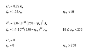
Form-drag roughness is primarily a function of the ripple properties and calculated as (Soulsby 1997): | |||
[[Image:12m2d.png|155px|]] | |||
{|border="0" cellspacing="2" width="100%" | {|border="0" cellspacing="2" width="100%" | ||
| | |||
|align = "right"|(45) | |||
|} | |||
in which ''H''<sub>''r''</sub> = ripple height, and ''L''<sub>''r''</sub> = ripple length, which are computed from: | |||
| | [[Image:14m2g.png|150px|]] | ||
{|border="0" cellspacing="2" width="100%" | |||
| | | | ||
|align = "right"|(46) | |||
|} | |||
for a current (Soulsby 1997) and from: | |||
| | [[Image:15m2d.png|285px|]] | ||
| | |||
| | {|border="0" cellspacing="2" width="100%" | ||
| | |||
|align = "right"|(47) | |||
|} | |||
for waves (van Rijn 1993), where [[Image:17m2d.png|20px|]] | |||
= mobility parameter that is defined by: | |||
| | [[Image:16m2d.png|150px|]] | ||
{|border="0" cellspacing="2" width="100%" | |||
| | | | ||
|align = "right"|(48) | |||
|} | |||
and ''s'' = specific density given by: | |||
[[Image:18m2d.png|90px|]] | |||
| | {|border="0" cellspacing="2" width="100%" | ||
| | |||
|align = "right"|(49) | |||
|} | |||
The sediment-related roughness is given by Wilson (1966, 1989): | |||
| | [[Image:M2D.pic2.png|90px|]] | ||
| | |||
{|border="0" cellspacing="2" width="100%" | |||
| | | | ||
|align = "right"|( SEQ Ch4Eq \* MERGEFORMAT 50) | |||
|} | |||
where [[Image:M2D.pic3.png|20px|]]= Shields parameter for current or waves (''i ''= ''c'', ''w'', respectively, for current and waves). Expressions for the Shields parameter for currents[[Image:M2D.pic3.png|20px|]]and for waves[[Image:M2D.pic3.png|20px|]]are given by: | |||
| | [[Image:M2D.pic4.png|180px|]] | ||
| | |||
{|border="0" cellspacing="2" width="100%" | |||
| | |||
|align = "right"|(51) | |||
|- | |- | ||
| | |||
|align = "right"|(52) | |||
|} | |||
Equation 50 has to be solved simultaneously with the expression for the shear stress, because the roughness depends on the stress. Explicit predictive equations were developed using approximating polynomials to the exact solution avoid time-consuming iteration in calculating the shear stress. | |||
Based on the roughness estimate, friction factors for current ''f''<sub>''c''</sub> and waves ''f''<sub>''w''</sub> are separately computed according to Soulsby (1997) and Swart (1974), respectively as: | |||
{|border="0" cellspacing="2" width="100%" | |||
| | | | ||
[[Image:M2D.pic5.png|180px|]] | |||
|= | |align = "right"|(53) | ||
| | |||
|- | |- | ||
|[[Image:M2D.pic6.png|350px|]] | |||
| | |align = "right"|(54) | ||
|} | |||
where [[Image:M2D.pic7.png|15px|]]=Von Karman constant (taken to be 0.4). Shear stress from the current is given by: | |||
{|border="0" cellspacing="2" width="100%" | |||
| | | | ||
[[Image:M2D.pic8.png|130px|]] | |||
|= | |align = "right"|(55) | ||
|} | |||
| | whereas the maximum shear stress from the waves is estimated from: | ||
{|border="0" cellspacing="2" width="100%" | |||
| | |||
| | |||
| | | | ||
[[Image:M2D.pic9.png|130px|]] | |||
|align = "right"|(56) | |||
| | |||
| | |||
|= | |||
| | |||
|} | |} | ||
and the mean shear stress is obtained from: | |||
{|border="0" cellspacing="2" width="100%" | {|border="0" cellspacing="2" width="100%" | ||
| | | | ||
[[Image:M2D.pic10.png|110px|]] | |||
|align = "right"|( | |align = "right"|(57) | ||
|} | |} | ||
where a sinusoidal wave is assumed. The corresponding shear velocities for current and waves, respectively, are defined as: | |||
{|border="0" cellspacing="2" width="100%" | |||
| | |||
[[Image:M2D.pic11.png|90px|]] | |||
|align = "right"|(58) | |||
|} | |||
for the current, and: | |||
{|border="0" cellspacing="2" width="100%" | {|border="0" cellspacing="2" width="100%" | ||
| | | | ||
[[Image:M2D.pic12.png|90px|]] | |||
| | |align = "right"|(59) | ||
| | |||
|= | |||
| | |||
|} | |} | ||
for the waves (based on the maximum shear stress). | |||
====Bed load==== | |||
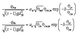
A general transport formula for bed load | |||
[[Image:M2D.pic16.png|15px|]] | |||
under combined waves and current was developed by Camenen and Larson (2005): | |||
{|border="0" cellspacing="2" width="100%" | {|border="0" cellspacing="2" width="100%" | ||
| | | | ||
[[Image:M2D.pic13.png|300px|]] | |||
|align = "right"|( | |align = "right"|(60) | ||
|} | |} | ||
where subscripts ''w'' and ''n'' refer to the wave direction and the direction normal to the waves, respectively, ''a'' and ''b'' are coefficients, and | |||
where | [[Image:M2D.pic14.png|35px|]] | ||
and | |||
[[Image:M2D.pic15.png|30px|]] | |||
are the mean and maximum Shields parameter for waves and current combined, respectively, not including the bed form roughness. The coefficient ''a''<sub>''n''</sub> = 12 for the transport component normal to the wave direction (current-driven transport). The coefficient ''b'' describes initiation of motion and is specified as ''b'' = 4.5. | |||
The quantities | |||
[[Image:M2D.pic17.png|20px|]] | |||
and | |||
[[Image:M2D.pic18.png|20px|]] | |||
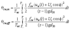
represent the net contribution of the shear stress to the transporting velocity during a wave cycle in the direction parallel and normal to the waves, respectively, defined as: | |||
{|border="0" cellspacing="2" width="100%" | {|border="0" cellspacing="2" width="100%" | ||
| | | | ||
[[Image:M2D.pic19.png|130px|]] | |||
|align = "right"|( | |align = "right"|(61) | ||
|} | |} | ||
in which: | |||
in which | |||
{|border="0" cellspacing="2" width="100%" | {|border="0" cellspacing="2" width="100%" | ||
| | | | ||
[[Image:M2D.pic20.png|280px|]] | |||
|align = "right"|( | |align = "right"|(62) | ||
|} | |} | ||
and | |||
{|border="0" cellspacing="2" width="100%" | {|border="0" cellspacing="2" width="100%" | ||
| | | | ||
[[Image:M2D.pic21.png|180px|]] | |||
|align = "right"|( | |align = "right"|(63) | ||
|} | |} | ||
where ''T''<sub>''wc''</sub> = period of positive flow, ''T''<sub>''wt''</sub> = period of negative flow, and ''u''<sub>''w''</sub> = time-varying horizontal bottom orbital velocity ( | |||
where | ). Analytical solutions to these equations are available for simple expressions of ''u''<sub>''w''</sub>. The friction factor for combined wave and current flow is calculated from Madsen and Grant (1976): | ||
= | |||
= | |||
{|border="0" cellspacing="2" width="100%" | {|border="0" cellspacing="2" width="100%" | ||
| | | | ||
[[Image:M2D.pic22.png|180px|]] | |||
|align = "right"|( | |align = "right"|(64) | ||
|} | |} | ||
where | |||
The | [[Image:M2D.pic23.png|100px|]] | ||
and ''f''<sub>''c''</sub> and ''f''<sub>''w''</sub> are the friction coefficients for current only and waves only, respectively, not including the bed form roughness. The Shields parameter that determines the amount of sediment mobilized for transport is obtained as: | |||
{|border="0" cellspacing="2" width="100%" | {|border="0" cellspacing="2" width="100%" | ||
| | | | ||
[[Image:M2D.pic24.png|250px|]] | |||
|align = "right"|( | |align = "right"|(65) | ||
|} | |} | ||
and the Shields parameter applied in the initiation of motion term is: | |||
{|border="0" cellspacing="2" width="100%" | {|border="0" cellspacing="2" width="100%" | ||
| | | | ||
[[Image:M2D.pic25.png|250px|]] | |||
|align = "right"|(66) | |||
|} | |||
where | |||
[[Image:M2D.pic26.png|25px|]] | |||
and | |||
[[Image:M2D.pic27.png|25px|]] | |||
are the Shields parameters for current only and waves only, respectively, and the index ''m'' denotes the mean value. For sinusoidal waves, | |||
[[Image:M2D.pic28.png|90px|]]. | |||
Values of the transport rate coefficients were obtained through calibration against a large data set from laboratory and field experiments involving a mean current, oscillatory waves (sinusoidal and asymmetric), and combined waves and current. A wide range of current and wave velocities, grain sizes, and roughness conditions were covered in this combined data set. The following relationship was developed for the transport coefficient in the wave direction (Camenen and Larson 2005): | |||
{|border="0" cellspacing="2" width="100%" | |||
| | |||
[[Image:M2D.pic29.png|100px|]] | |||
|align = "right"|(67) | |||
|} | |||
In many applications, the waves are assumed to be sinusoidal, having no asymmetry. Thus, the contribution to the transporting velocity from the waves is negligible, implying that only the current moves the material. Waves are still important for mobilization of the sediment. For such conditions, Equation 60 simplifies to: | |||
{|border="0" cellspacing="2" width="100%" | |||
| | |||
[[Image:M2D.pic30.png|240px|]] | |||
|align = "right"|(68) | |||
|} | |||
where the transport ''q''<sub>''bc''</sub> is obtained in the direction of the current, and the transport normal to the current is zero. (There is no velocity component to move the material in this direction.) | |||
====Suspended load==== | |||
The suspended load ''q''<sub>''s''</sub> is calculated based on the assumptions of an exponential concentration profile and a constant velocity over the water column to yield (Camenen and Larson 2006): | |||
{|border="0" cellspacing="2" width="100%" | |||
|[[Image:M2D.pic35.png|180px|]] | |||
|align = "right"|( | |align = "right"|(69) | ||
|} | |} | ||
where ''R'' is the | where ''w''<sub>''f</sub> '' = sediment fall speed, ''c''<sub>''R''</sub> = reference concentration, and[[Image:M2D.pic32.png|10px|]] = sediment diffusivity (or mixing coefficient). The transport ''q''<sub>''s''</sub> is taken to be in the direction of the current because the waves are assumed to produce a zero net drift and not contribute to the transport. In the calculation of ''c''<sub>''R''</sub> and[[Image:M2D.pic32.png|10px|]] , the total shear stress should be applied, including the bed form roughness. The reference concentration is given by: | ||
{|border="0" cellspacing="2" width="100%" | {|border="0" cellspacing="2" width="100%" | ||
| | |[[Image:M2D.pic36.png|180px|]] | ||
|align = "right"|( | |align = "right"|(70) | ||
|} | |} | ||
where | where the coefficient[[Image:M2D.pic37.png|25px|]] is determined by the following relationship: | ||
{|border="0" cellspacing="2" width="100%" | {|border="0" cellspacing="2" width="100%" | ||
| | |[[Image:M2D.pic38.png|180px|]] | ||
|align = "right"|( | |align = "right"|(71) | ||
|} | |} | ||
and the dimensionless grain size is defined by[[Image:M2D.pic39.png|150px|]] | |||
. The sediment diffusivity is related to the energy dissipation according a generalization of the treatment of Battjes (1975): | |||
{|border="0" cellspacing="2" width="100%" | |||
|[[Image:M2D.pic40.png|120px|]] | |||
|align = "right"|(72) | |||
|} | |||
where ''D''<sub>''e''</sub> is a total effective dissipation given by: | |||
{|border="0" cellspacing="2" width="100%" | |||
|[[Image:M2D.pic41.png|180px|]] | |||
|align = "right"|(73) | |||
|} | |||
in which ''k''<sub>''c''</sub>, ''k''<sub>''w''</sub>, and ''k''<sub>''b''</sub> are coefficients. The dissipations from bottom friction due to current ''D''<sub>''ec''</sub> and from bottom friction due to waves ''D''<sub>''ew''</sub> are expressed as: | |||
{|border="0" cellspacing="2" width="100%" | {|border="0" cellspacing="2" width="100%" | ||
| | |||
|align = "right"|( | |[[Image:M2D.pic42.png|120px|]] | ||
| | |||
|align = "right"|(74) | |||
|- | |||
|align = "right"|( | |[[Image:M2D.pic43.png|120px|]] | ||
|align = "right"|(75) | |||
|} | |} | ||
and the dissipation due to wave breaking ''D''<sub>''eb''</sub> is directly provided from a wave transformation model (e.g., STWAVE. WABED). The coefficient ''k''<sub>''b''</sub> corresponds to an efficiency factor and was found to be 0.017, whereas ''k''<sub>''c''</sub> and ''k''<sub>''w''</sub> are related to the Schmidt number that expresses the ratio between diffusivity of sediment and water (i.e., momentum). These two coefficients are given by: | |||
{|border="0" cellspacing="2" width="100%" | {|border="0" cellspacing="2" width="100%" | ||
| | |||
|align = "right"|( | |[[Image:M2D.pic44.png|100px|]] | ||
|align = "right"|(76) | |||
|} | |} | ||
where[[Image:M2D.pic45.png|20px|]]= Schmidt number and the subscript ''i'' = ''c'' or ''w'' denotes current and waves, respectively. The Schmidt number is calculated from the empirical relationships: | |||
{|border="0" cellspacing="2" width="100%" | {|border="0" cellspacing="2" width="100%" | ||
| | |||
|align = "right"|( | |[[Image:M2D.pic46.png|400|]] | ||
|align = "right"|(77) | |||
|} | |} | ||
for waves | |||
where ''A''<sub>''1''</sub> = 0.7 and ''A''<sub>''2''</sub> = 3.6 for current, and ''A''<sub>''1''</sub> = 0.09 and ''A''<sub>''2''</sub> = 1.4 for waves. In the case of coexistent waves and current, a weighted Schmidt number is applied according to: | |||
{|border="0" cellspacing="2" width="100%" | {|border="0" cellspacing="2" width="100%" | ||
| | |||
|align = "right"|( | |[[Image:M2D.pic47.png|250px|]] | ||
|align = "right"|(78) | |||
|} | |} | ||
and | |||
for both waves and current. | |||
Bed load and suspended load transport rates are set to zero at the beginning of the simulation, then updated at each sediment transport time step. | |||
The | ===Advection-Diffusion Equation=== | ||
Calculations of suspended load and bed load are conducted separately through solution of the AD equation for suspended load. This method calculates the suspended load in the water column through the lateral and vertical movement of the sediment. | |||
====Basic equations==== | |||
Sediment transport consists of two components, bed load and suspended load. The bed load and suspended load transport rate formulas are based on the local shear stress. However, in the situation where the suspended sediment concentration rapidly changes in time and space, such as at a river mouth, inlet entrance, navigation channel, and in the vicinity of structures, the suspended load cannot be determined solely by the local forcing conditions. In this case, suspended sediment concentration is governed by the AD equation. | |||
The AD equation implemented in CMS-M2D is obtained from the continuity of depth-averaged suspended sediment transport (Figure 2) as: | |||
{|border="0" cellspacing="2" width="100%" | {|border="0" cellspacing="2" width="100%" | ||
| | |||
|align = "right"|( | |[[Image:M2D.pic48.png|400px|]] | ||
|align = "right"|(79) | |||
|} | |} | ||
in which | |||
{|border="0" cellspacing="2" width="100%" | {|border="0" cellspacing="2" width="100%" | ||
| | |||
| | |'' | ||
|C'' | |||
|= | |||
|depth-averaged sediment concentration | |||
|- | |- | ||
| | |||
| | |'' | ||
| | |||
|d'' | |||
|= | |||
| | |total depth (= ''h''<nowiki>+</nowiki>[[Image:M2D.pic49.png|10px|]] ) | ||
|- | |- | ||
= | |'' | ||
|h | |||
|''= | |||
|still-water depth | |||
|- | |||
| | | | ||
==== | |[[Image:M2D.pic49.png|10px|]] | ||
|= | |||
|deviation of the water-surface elevation from the still-water level | |||
|- | |||
|'' | |||
|t | |||
|''= | |||
|time | |||
|- | |||
|'' | |||
|q''<font size = "1">''x | |||
|''</font>= | |||
|flow per unit width parallel to the x''-''axis (= ''ud'') | |||
|- | |||
|'' | |||
|q''<font size = "1">''y | |||
|''</font>= | |||
|flow per unit width parallel to the y-axis (= ''vd'') | |||
| | |- | ||
| | |'' | ||
| | |u | ||
|''= | |||
|depth-averaged current velocity parallel to the x-axis | |||
|- | |||
|'' | |||
| | |v | ||
|''= | |||
|depth-averaged current velocity parallel to the y-axis | |||
|- | |||
|'' | |||
| | |K''<font size = "1">''x | ||
| | |''</font>= | ||
|sediment diffusion coefficient for the ''x ''direction | |||
|- | |||
|'' | |||
| | |K''<font size = "1">''y | ||
| | |''</font>= | ||
| | |sediment diffusion coefficient for the ''y ''direction | ||
|- | |||
|'' | |||
|P'' | |||
| | |= | ||
| | |sediment pick-up rate (upward sediment flux) | ||
| | |- | ||
|'' | |||
|D'' | |||
| | |= | ||
| | |sediment deposition rate (downward sediment flux) | ||
|} | |} | ||
The suspended sediment concentration can be solved from Equation 79 at a sediment transport time step. | |||
[[Image:M2D.pic50.png|thumb|center|400px|Figure 2]] | |||
[[Image:Figure2|framed|none|500px|Figure2. Definition of continuity (conservation of volume) of sediment transport]] | |||
Bed level change is obtained from the sediment continuity equation: | |||
{|border="0" cellspacing="2" width="100%" | {|border="0" cellspacing="2" width="100%" | ||
| | | | ||
| | |[[Image:M2D.pic51.png|250px]] | ||
| | |align = "right"|(80) | ||
| | |} | ||
where ''q''<sub>''bx''</sub> = bed load transport rate parallel to the x-axis, ''q''<sub>''by''</sub> = bed load transport rate parallel to the y-axis, and ''p'' = porosity of sediment. | |||
and the | In Equation 80, the terms | ||
[[Image:M2D.pic52.png|100px]] include the bed load component, and the term ''P-D'' corresponds to the suspended load component. Figure 2 shows the definition of sediment continuity in a water column, where ''q''<sub>''sx''</sub> and ''q''<sub>''sy''</sub> are the suspended transport rate in the ''x'' and ''y'' directions, respectively, and ''a ''is the height of the bed load layer. The transport rates ''q''<sub>''sx''</sub> and ''q''<sub>''sy''</sub> may be defined as follows from Equation 79: | |||
{|border="0" cellspacing="2" width="100%" | {|border="0" cellspacing="2" width="100%" | ||
| | |[[Image:M2D.pic53.png|150px]] | ||
|align = "right"|( | |align = "right"|(81) | ||
| | |- | ||
|[[Image:M2D.pic54.png|150px]] | |||
= | |align = "right"|(82) | ||
|} | |||
Sediment concentration and bed load and suspended load transport rates are set to zero at the beginning of the simulation, then updated at each sediment transport time step. | |||
|align = "right"|( | ====Pick-up and deposition rates==== | ||
The AD model calculates the bed level change due to suspended load from the difference between pick-up rate and deposition rate in Equation 80. The pick-up rate and the deposition rate are also applied as the bottom boundary condition in Equation 79. The boundary conditions are specified at an arbitrary level ''a'' above the mean bed level: | |||
{|border="0" cellspacing="2" width="100%" | |||
|[[Image:M2D.pic55.png|150px]] | |||
|align = "right"|(83) | |||
|- | |||
|[[Image:M2D.pic56.png|75px]] | |||
|align = "right"|(84) | |||
|} | |||
where ''c'' = equilibrium concentration of suspended sediment at a given elevation, and ''z'' = vertical coordinate. Both ''c''<sub>''a''</sub> and ''c''<sub>0</sub> are reference concentrations defined at ''z ''= ''a''. Because the upward flux of sediment depends on the bed shear stress, ''c''<sub>''a''</sub> is determined from the bed shear stress calculated from the local hydrodynamic conditions. Representation of ''c''<sub>''a''</sub> within CMS-M2D is dependent on selection of either the van Rijn or Lund-CIRP models. The downward sediment flux depends on the concentration in the upper water column; therefore, ''c''<sub>0</sub> is specified from solution of Equation 79. | |||
Assuming that the suspended concentration is in equilibrium | |||
[[Image:M2D.pic57.png|300px]] | |||
, then the basic equation for suspended sediment concentration can be written: | |||
{|border="0" cellspacing="2" width="100%" | |||
|[[Image:M2D.pic58.png|155px]] | |||
|align = "right"|(85) | |||
|} | |||
This equation can be solved analytically by applying an appropriate mixing coefficient | |||
[[Image:M2D.pic32.png|8px]] | |||
, and the vertical profile of suspended concentration is obtained in the following form: | |||
{|border="0" cellspacing="2" width="100%" | |||
|[[Image:M2D.pic59.png|125px]] | |||
|align = "right"|(86) | |||
|} | |||
where ''F''(''z'') is a function of the vertical concentration distribution. The relationship between the reference concentration ''c''<sub>0</sub> and the depth-averaged concentration ''C'' is: | |||
{|border="0" cellspacing="2" width="100%" | |||
|[[Image:M2D.pic60.png|150px]] | |||
|align = "right"|(87) | |||
|} | |||
Thus, ''c''<sub>0</sub> may be written in the following form by introducing a conversion function <sub>''d''</sub>: | |||
{|border="0" cellspacing="2" width="100%" | |||
|[[Image:M2D.pic61.png|150px]] | |||
|align = "right"|(88) | |||
|} | |||
The bed level change due to suspended load is based upon the difference of the two types of reference concentration: | |||
{|border="0" cellspacing="2" width="100%" | |||
|[[Image:M2D.pic62.png|150px]] | |||
|align = "right"|(89) | |||
|} | |} | ||
This equation implies that erosion occurs if'' c''<sub>''a''</sub> <nowiki>></nowiki> ''c''<sub>0</sub>, and accretion occurs if ''c''<sub>''a''</sub> <nowiki><</nowiki> ''c''<sub>0</sub>. | |||
In the AD model, three methods of specifying ''c''<sub>''a''</sub> and ''c''<sub>0</sub> (that is, | |||
[[Image:M2D.pic63.png|20px]])are implemented. Two of the methods are based on the van Rijn formula (van Rijn 1985) and one on the Lund-CIRP formula (Camenen and Larson 2006). Table 1 summarizes general features of the methods. | |||
<u>van Rijn formula</u> | |||
The reference concentration ''c''<sub>''a''</sub> in the van Rijn formula is given by: | |||
{|border="0" cellspacing="2" width="100%" | {|border="0" cellspacing="2" width="100%" | ||
|[[Image:M2D.pic64.png|250px]] | |||
|align = "right"|(90) | |||
|} | |||
where ''a'' = reference height and | |||
[[Image:M2D.pic68.png|10px]]<sub>''s'',max</sub> = maximum bed shear stress given by Equation 38. | |||
{|border="2" cellspacing="0" cellpadding="4" width="75%" | |||
|colspan = "4"|'''Features of Calculation of Pick-up and Deposition Rates''' | |||
|- | |||
|<font size = "2">'''Method'''</font> | |||
|<font size = "2">'''Reference Concentration'''</font> | |||
|<font size = "2">'''Conversion Parameter'''</font> | |||
|<font size = "2">'''Comments'''</font> | |||
|- | |||
|Exponential Profile | |||
|Eq. 90 | |||
|Eq. 104 and 105 | |||
|Fast computation.<br>Tends to overestimate sediment transport rate.<br>Can be used for some tests. | |||
|- | |||
|Van Rijn Profile | |||
|Eq. 90 | |||
|Solves Eq. 85 numerically with Eq. 103 (Runge-Kutta 4<sup>th</sup>) | |||
|Requires substantial computing time.<br>Provides the same results as van Rijn (1985). | |||
|- | |||
|Lund-CIRP Profile | |||
|Eq. 70 | |||
|Eq. 104 and 72 | |||
|Fast computation.<br>Newly developed sediment transport formula. | |||
|} | |||
The current-related shear stress is calculated from: | |||
{|border="0" cellspacing="2" width="100%" | |||
|[[Image:M2D.pic65.png|200px]] | |||
|align = "right"|(91) | |||
|} | |||
The wave-related shear stress is given as: | |||
{|border="0" cellspacing="2" width="100%" | |||
|[[Image:M2D.pic66.png|100px]] | |||
|align = "right"|(92) | |||
|- | |||
|[[Image:M2D.pic67.png|180px]] | |||
|align = "right"|(93) | |||
|} | |||
where | |||
= roughness height defined as: | |||
{|border="0" cellspacing="2" width="100%" | |||
|[[Image:M2D.pic69.png|150x]] | |||
|align = "right"|(94) | |||
|} | |||
in which ''k''<sub>''sd''</sub> and ''k''<sub>''ss''</sub> are calculated from Equations 37 and 50, respectively. | |||
| | Bed concentration in the van Rijn model is defined at the height ''a'' as: | ||
{|border="0" cellspacing="2" width="100%" | |||
|align = "right"|( | |[[Image:M2D.pic70.png|200px]] | ||
|align = "right"|(95) | |||
|} | |||
where ''H''<sub>''r''</sub> = ripple height. If ripples are present, the total roughness height is modified as: | |||
{|border="0" cellspacing="2" width="100%" | |||
|[[Image:M2D.pic71.png|100px]] | |||
|align = "right"|(96) | |||
|} | |} | ||
where,'' k''<sub>''sf</sub> '' = 20(''H''<sub>''r''</sub><sup>2</sup>''/L''<sub>''r''</sub>) is specified for the van Rijn formula, and ''k''<sub>''sf''</sub> '' ''= 7.5(''H''<sub>''r''</sub><sup>2</sup>''/L''<sub>''r''</sub>) is specified for the Lund-CIRP formula. The ripple dimension is obtained by selecting the largest ripple height for the case of current or waves (Equations 46 and 47). | |||
for | The conversion parameter [[Image:M2D.pic63.png|20px]] to determine ''c''<sub>0</sub> is obtained from the vertical mixing coefficient. Van Rijn (1985) proposed a distribution of the mixing coefficients for only current or waves according to Figure 3. The current-related mixing coefficient is given by: | ||
{|border="0" cellspacing="2" width="100%" | |||
|[[Image:M2D.pic72.png|350px]] | |||
|align = "right"|(97) | |||
|} | |||
where ''u''<sub>''*c''</sub> = current-related bed shear velocity expressed as: | |||
{|border="0" cellspacing="2" width="100%" | |||
|[[Image:M2D.pic74.png|200px]] | |||
|align = "right"|(98) | |||
|} | |||
and[[Image:M2D.pic75.png|20px]]is a coefficient obtained from: | |||
{|border="0" cellspacing="2" width="100%" | |||
|[[Image:M2D.pic76.png|300px]] | |||
|align = "right"|(99) | |||
|} | |||
[[Image:M2D.pic77.png|650px]] | |||
Figure3. Vertical distributions of mixing coefficient due to current and waves | |||
The wave-related mixing coefficient is: | |||
{|border="0" cellspacing="2" width="100%" | |||
=== | |[[Image:M2D.pic78.png|500px]] | ||
|align = "right"|(100) | |||
|} | |||
where | |||
{|border="0" cellspacing="2" width="100%" | |||
|[[Image:M2D.pic79.png|175px]] | |||
|align = "right"|(101) | |||
|- | |||
=== | |[[Image:M2D.pic80.png|275px]] | ||
|align = "right"|(102) | |||
|} | |||
in which the parameter | |||
= height from the bed given by | |||
, ''H'' = significant wave height, and ''T'' = significant wave period. If waves and current coexist, the combined mixing coefficient is given by: | |||
{|border="0" cellspacing="2" width="100%" | {|border="0" cellspacing="2" width="100%" | ||
|[[Image:M2D.pic81.png|125px]] | |||
| | |align = "right"|(103) | ||
|align = "right"|( | |||
|} | |} | ||
By applying the expression for [[Image:M2D.pic32.png|10px]] | |||
<sub>''cw''</sub>, the concentration profile can be derived from Equation 85, and the conversion parameter[[Image:M2D.pic63.png|15px]]calculated. In the AD-model based on the van Rijn equations, two methods are implemented to calculate | |||
[[Image:M2D.pic63.png|15px]]. One is based on an exponential profile employing a depth-averaged mixing coefficient[[Image:M2D.pic82.png|25px]], and the other uses the original van Rijn profile, where the [[Image:M2D.pic63.png|15px]]is obtained by numerical integration of Equation 85. Assuming an exponential profile of suspended sediment concentration,[[Image:M2D.pic63.png|15px]]is obtained analytically as: | |||
{|border="0" cellspacing="2" width="100%" | {|border="0" cellspacing="2" width="100%" | ||
|[[Image:M2D.pic83.png|225px]] | |||
|align = "right"|(104) | |||
|} | |||
where | |||
{|border="0" cellspacing="2" width="100%" | |||
|[[Image:M2D.pic84.png|170px]] | |||
|align = "right"|(105) | |||
|} | |||
<u>Lund-CIRP formula</u> | |||
Reference concentration and sediment diffusivity calculated by the Lund-CIRP formula may also be applied in the AD-model. The formulas used for ''c''<sub>''R''</sub> and ε are presented in the section describing the Lund-CIRP formula. | |||
|= | ====Horizontal diffusion coefficient==== | ||
Horizontal diffusion coefficients ''K''<sub>''x''</sub> and ''K''<sub>''y''</sub> for the depth-averaged sediment concentration in the AD equation are calculated by the equation proposed by Elder (1959): | |||
{|border="0" cellspacing="2" width="100%" | |||
|[[Image:M2D.pic85.png|125px]] | |||
|align = "right"|(106) | |||
|} | |||
In the surf zone, waves contribute significantly to lateral mixing, and the eddy viscosity coefficient is expected to be a function of the wave properties. For the horizontal diffusion coefficients for AD equation, surf zone mixing proposed by Kraus and Larson (1991) is applied as well as for hydrodynamic calculation. | |||
{|border="0" cellspacing="2" width="100%" | |||
|[[Image:M2D.pic86.png|75px]] | |||
|align = "right"|(107) | |||
|} | |||
where[[Image:M2D.pic87.png|15px]]describes the lateral mixing below trough level (Smith, Larson, and Kraus, 1993) and is expressed as (Kraus and Larson 1991): | |||
{|border="0" cellspacing="2" width="100%" | |||
|[[Image:M2D.pic88.png|100px]] | |||
|align = "right"|(108) | |||
|} | |||
where [[Image:M2D.pic89.png|15px]]= empirical coefficient representing the lateral mixing strength. | |||
| | The transition between surf zone diffusion and oceanic diffusion seaward of the breakpoint is represented in CMS-M2D by a weighted mixing coefficient specified as: | ||
{|border="0" cellspacing="2" width="100%" | |||
|[[Image:M2D.pic90.png|175px]] | |||
|align = "right"|(109) | |||
|} | |||
where the weighting parameter[[Image:M2D.pic91.png|25px]]is given by: | |||
{|border="0" cellspacing="2" width="100%" | |||
|[[Image:M2D.pic92.png|125px]] | |||
|align = "right"|(110) | |||
|} | |||
|- | ====Bed load transport rate==== | ||
Bed load transport rate may be calculated with the van Rijn (1998) or Lund-CIRP (Camenen and Larson 2005) formula. In the van Rijn formula, bed load transport rate is obtained from, not including bed roughness: | |||
{|border="0" cellspacing="2" width="100%" | |||
|[[Image:M2D.pic93.png|250px]] | |||
|align = "right"|(111) | |||
|} | |||
The Lund-CIRP formula for bed load is described previously in this chapter. | |||
===Scaling Factors for Bed Load and Suspended Load Transport Rates=== | |||
Adjustments to the bed load and suspended load transport rates can be assigned for both the Lund-CIRP total load formulation | |||
and the AD equation. Scaling factors are applied directly to transport rate values as coefficients independently for the bed | |||
load transport rate and for the suspended load transport rate. Thus, the bed load transport rate can be scaled separately | |||
from the suspended load transport rate. Recommended ranges for the scaling factors are 0.1 to 4. A scaling factor of 1 will | |||
not modify the transport rate, and this value is the default. Values less than 1 will reduce the transport rate, and values | |||
greater than 1 will increase it. Scaling factors are sometimes found necessary because of uncertainties in forcing and initial conditions, allowing adjustment of model predictions of sediment transport rates and morphology change to observations. | |||
===Sediment Continuity Equation=== | |||
Depth change for the total load formulations and for bed load transport from the AD equation is calculated by the sediment continuity equation, in which time-averaged transport rates are applied. This approach requires that two time intervals be defined, one over which to compute instantaneous transport rates ''dt''<sub>''sed''</sub> and the other over which to compute averaged transport rates and morphology change ''dt''<sub>''morph''</sub>. Directional instantaneous transport rates [[Image:M2D.pic96.png|35px|]]and[[Image:M2D.pic97.png|35px|]] are calculated at intervals of ''dt''<sub>''sed''</sub> and averaged over the time interval ''dt''<sub>''morph''</sub> to obtain the time-averaged transport rates [[Image:M2D.pic94.png|35px|]] and | |||
| | [[Image:M2D.pic95.png|35px|]] | ||
for the x and y directions, respectively. Enhancement of down-slope transport and reduction of up-slope transport rates is accomplished by calculation of modified time-averaged transport rates | |||
[[Image:M2D.pic98.png|35px|]] and [[Image:M2D.pic99.png|35px|]]as (Watanabe 1987): | |||
{|border="0" cellspacing="2" width="100%" | |||
|[[Image:M2D.pic100.png|175px|]] | |||
|align = "right"|(112) | |||
|- | |- | ||
|'' | |[[Image:M2D.pic101.png|175px|]] | ||
|align = "right"|(113) | |||
|} | |||
in which [[Image:M2D.pic103.png|17px|]] | |||
= empirical slope coefficient with typical range of 5 to 30, and [[Image:M2D.pic104.png|23px|]] | |||
is the time- | |||
averaged transport rate. These formulations add an effective diffusion of transport to the continuity equation for bed change. | |||
The sediment continuity equation is solved to compute depth change at the time interval ''dt''<sub>''morph''</sub> and for total load formulations is given by: | |||
| | {|border="0" cellspacing="2" width="100%" | ||
|[[Image:M2D.pic105.png|225px|]] | |||
|align = "right"|(114) | |||
|} | |||
At forcing boundaries, the gradient in transport rate across the boundary cell is set to zero. | |||
For the AD-model, the sediment continuity equation is provided by Equation 80. The time intervals to compute instantaneous transport rates and to compute averaged transport rates and morphology change are consistent with those applied in the total load model, that is, ''dt''<sub>''sed''</sub> and ''dt''<sub>''morph''</sub> respectively. Also, the bed load components in Equation 80 are modified by the slope effect as: | |||
{|border="0" cellspacing="2" width="100%" | |||
| | |||
|[[Image:M2D.pic106.png|200px|]] | |||
|align = "right"|(115) | |||
|- | |- | ||
| | |||
|[[Image:M2D.pic107.png|200px|]] | |||
|align = "right"|(116) | |||
|- | |||
| | Where[[Image:M2D.pic108.png|100px|]] Finally, the sediment continuity equation is solved to compute depth change at the time interval ''dt''<sub>''morph''</sub> and is rewritten as: | ||
| | {|border="0" cellspacing="2" width="100%" | ||
| | |||
|[[Image:M2D.pic109.png|220px|]] | |||
|align = "right"|(117) | |||
|} | |||
which contains both bed load and suspended load components. At forcing boundaries, the gradient intransport rate across the boundary cell is set to zero. | |||
===Hard-Bottom Methodology=== | |||
Representation of hard (non-erodible) substrate provides the capability to simulate mixed bottom types within a single simulation. The default bottom type in CMS-M2D is erodible, meaning that sediment is available to be transported from that area. Areas having hard bottom are specifically designated as such in the model, and the depth of the hard substrate is specified, allowing representation of either exposed or sediment-covered hard bottom. The one-dimensional (1D) hard-bottom calculation approach applied in the GENESIS shoreline change model (Hanson 1989; Hanson and Kraus 1989) to represent the control of seawalls on shoreline evolution (Hanson and Kraus 1985, 1986) was extended to two dimensions and implemented in CMS-M2D (Hanson and Militello 2005). | |||
The presence of hard bottom exerts a constraint on water depth because the bottom cannot erode. Representation of hard bottom applies an adjustment to the potential transport rates (calculated by a transport formulation with no restriction) to account for the presence of hard substrate. Treatment of hard bottom was developed to satisfy the following four properties: | |||
| | {|border="0" cellspacing="2" width="100%" | ||
| | |''a''. | ||
|Areas having hard bottom cannot erode below the level of the hard substrate. | |||
|- | |- | ||
|'' | |''b''. | ||
|Sediment volume is conserved. | |||
| | |- | ||
|'' | |''c''. | ||
| | |The direction of sediment transport at a location with hard bottom is the same as that of the direction of potential local transport. | ||
|- | |- | ||
|'' | |''d''. | ||
| | |Correction to transport rates is always done in the direction of potential sediment transport. If hard bottom is exposed, the reduction in actual transport as compared to the situation without hard bottom is always transmitted to neighboring areas in the direction of transport as governed by the hydrodynamic forcing. | ||
| | |} | ||
The general procedure for treating hard bottom is: | |||
| | {|border="0" cellspacing="2" width="100%" | ||
| | |''a''. | ||
| | |Calculate sediment transport and morphology change without hard-bottom restriction. | ||
| | |- | ||
|'' | |''b''. | ||
|depth- | |Assess whether hard-bottom cells have eroded below the hard bottom depth. If so, apply a correction procedure that adjusts transport rates based on available sediment at hard-bottom cells and corrects depths so that the hard-bottom constraint is not violated. The correction procedure makes adjustments at all cells in which transport rates are controlled by hard bottom and can include adjustments at cells that do not have hard bottom. | ||
| | |} | ||
The correction procedure involves four steps: | |||
| | {|border="0" cellspacing="2" width="100%" | ||
|'' | |''a''. | ||
| | |Identify all cells that have transport at all four faces directed out of the cell, called "Minus4" cells. These Minus4 cells, if they exist, must constitute the first stage of corrections, as they are only <nowiki>’</nowiki>deliverers<nowiki>’</nowiki> of sediment to all adjacent cells, not <nowiki>’</nowiki>recipients<nowiki>’</nowiki> of material. | ||
|- | |- | ||
|'' | |''b''. | ||
|If the hard bottom is exposed, all transport rates out of the Minus4 cells are reduced. A list of all adjacent cells, with or without hard bottom, that are influenced by exposed hard-bottom cells is generated for later correction to depths and transport rates. | |||
| | |- | ||
|'' | |''c''. | ||
|sediment | |Depths at all adjacent cells are then recalculated to account for the reduced influx of sediment. Cells with hard bottom must then be checked for a possible violation of the hard-bottom constraint and corrected as necessary. For each corrected cell, all sediment transport rates out of the cell are in turn corrected, and each of the next generation of affected cells adjacent to it is added to the list of cells to be corrected. Transport rates into a cell are never changed (as it is an outgoing transport from the adjacent cell that is corrected in that cell). | ||
|- | |- | ||
|'' | |''d''. | ||
| | |After all cells have been checked, the process is repeated to make sure that the hard-bottom constraint is not violated in any cell. | ||
| | |} | ||
Corrections to transport rates and depths are based upon the potential transport rate and amount of sand available for erosion. If, after solution of the sediment continuity equation (Equation 114), the updated depth | |||
is greater than the hard-bottom level | |||
, the outgoing transport rates are corrected to match the criterion | |||
. Over one morphologic time step, the total amount of material | |||
, expressed as a vertical quantity that may leave the cell without violating the hard-bottom constraint is: | |||
| | {|border="0" cellspacing="2" width="100%" | ||
| | | | ||
| | |[[Image:M2D.pic111.png|220px|]] | ||
|= | |align = "right"|(118) | ||
|} | |} | ||
where ''q''<sub>''in''</sub> = total influx of sediment from the cell during the morphologic time step. The correction factor ''K'' is given as: | |||
{|border="0" cellspacing="2" width="100%" | {|border="0" cellspacing="2" width="100%" | ||
| | | | ||
| | |[[Image:M2D.pic112.png|150px|]] | ||
| | |align = "right"|(119) | ||
|} | |||
where ''q''<sub>''out''</sub> = total outflux of sediment from the cell during the morphologic time step. To ensure that [[Image:M2D.pic113.png|50px|]] | |||
ingoing transport rates are left unchanged, and outgoing transport rates are multiplied by the correction factor ''K''. | |||
| | A schematic example of the correction procedure is provided for a symmetric computational grid (Figure 4). The domain contains a 9-by-9 grid of calculation cells. Rows (parallel to the x-axis) are numbered 1 through 9, and columns (parallel to the y-axis) are indicated by A through I. Initial bathymetry level is specified to be[[Image:M2D.pic114.png|35px|]] at all cells, and the hard-bottom level is at [[Image:M2D.pic115.png|35px|]](units) at all cells (''z'' is positive downwards from the original bottom level at[[Image:M2D.pic114.png|35px|]]) | ||
Arrows across the cell walls indicate the initial (potential) transport rates. These are of three different magnitudes: 2 units/m/s (black arrows), 5 units/m/s (blue arrows), and 12 units/m/s (green arrows). For demonstration purposes we assume that the cell sizes in the x-direction and the y-direction are the same and that a transport rate of 1 unit/m/s during one time step corresponds to a bottom elevation change of 1. | |||
Numbers inside each cell indicate the potential depth change (positive numbers mean erosion) in each cell, which is a measure of the magnitude of the depth change if the hard bottom were not there. Thus, in each cell with a depth change that is greater than 5, the hard bottom is exposed. As a result, the actual depth change is limited to 5. Once this depth is reached, the transport out of the cell is reduced owing to limited sediment availability. | |||
In the model, this reduction is accomplished through a correction procedure. The following section explains how this correction is performed through three successive correction loops in a hierarchical and systematic order. | |||
[[Image:M2D.pic116.png|thumb|center|550px|]] | |||
Figure4. Schematic hard-bottom grid and potential transport rates | |||
'''Correction loop 1:''' | |||
{|border="0" cellspacing="2" width="100%" | {|border="0" cellspacing="2" width="100%" | ||
| | |||
| | |''a''. | ||
|Find cells with transport rates directed out of the cell through all four faces. These cells represent the ultimate starting points. Cell E5 is the only cell in this example having outward-directed transport rates through all four faces. | |||
|- | |- | ||
|''b''. | |||
|Calculate the new bottom level equaling 8 units, which means that the hard bottom at 5 units is exposed. | |||
| | |||
| | |||
|- | |- | ||
|''c''. | |||
| | |Reduce all transport rates out of cell E5 in proportion to the sediment deficit. The potential loss of sediment was 8 units while the available volume in cell E5 was 5 units. Thus, the outgoing transport rates will be reduced from 2 to 2 x 5/8 = 1.25 units/m/s. | ||
| | |||
|- | |- | ||
| | |''d''. | ||
| | |||
|Recalculate depths of all adjacent cells, D5, E4, F5, and E6, based on modified transport rates. | |||
|- | |- | ||
| | |''e''. | ||
| | |||
|Hard bottom is now exposed in cells E4 and E6. | |||
|- | |- | ||
|''f''. | |||
|Reduce transport rates out of these two cells (E4 and E6). | |||
|- | |- | ||
|''g''. | |||
|Recalculate depths of cells adjacent to E4 and E6 that receive sediment. These cells are D4, E3, F4 and D6, F6, E7. No additional hard-bottom cells are exposed. Thus, the deficit associated with cell E5 does not spread further. | |||
| | |||
|} | |} | ||
'''Correction loop 2:''' | |||
{|border="0" cellspacing="2" width="100%" | {|border="0" cellspacing="2" width="100%" | ||
|''h''. | |||
|Find ''start cells'' from where sand-deficit might spread by searching through the grid from one end to the other. ''Start cells'' are those that are located on a hard bottom, but do not receive sediment from any other hard-bottom cell. | |||
| | |||
where | |||
|- | |||
|''i''. | |||
= | |Find ''exposed cells'' (defined as cells where the hard bottom is exposed) and identify by flag IEXP = 1. Start the search in cell A1. This cell is exposed, but sediment is coming in from B1 that is also exposed. The direction of influence will be in the direction of transport, i.e., from B1 to A1. Thus, A1 cannot be a start cell. | ||
|- | |||
|''j''. | |||
|Next, proceed to cell A2. This cell is exposed but, as above, it is receiving sediment from cell A1, which is also exposed. Thus, cell A2 is not a start cell. | |||
|- | |||
|''k''. | |||
|The same situation prevails for all cells in the A column. Thus, no cells in the A column are start cells. | |||
|- | |||
|''l''. | |||
|Next, proceed to cell B1. This cell is exposed. It is only getting sand from B2, but that cell is not exposed, so no correction can come from there. Thus, cell B1 is a start cell. | |||
|- | |||
|''m''. | |||
as ( | |All remaining cells are checked the same way, and all start cells are added as necessary to the list of cells to be corrected (here referred to as the ''correction list''). | ||
|- | |- | ||
| | |''n''. | ||
| | |Correct the first cell in the correction list, cell B1. Add adjacent cells receiving sediment from B1 to the correction list, i.e., cells A1 and C1. | ||
|- | |||
|''o''. | |||
|Proceed through all start cells, correct outgoing transport rates, and add to the correction list all cells receiving sediment from the start cells. | |||
|} | |} | ||
'''Correction loop 3:''' | |||
| | {|border="0" cellspacing="2" width="100%" | ||
| | |''p''. | ||
| | |The next step is to examine all cells connected to start cells. Transport rates need to be corrected if hard bottom is exposed. Adjacent cells receiving sediment are added to the correction list at the next level of correction cells. | ||
| | |} | ||
Through this procedure, cells will always be corrected in a hierarchic order in which all cells of one level are corrected before proceeding to the next level. Corrections are always propagated in the direction of transport without ambiguity regarding which cell affects another. Figure 5 shows the final bathymetry where all (positive) depth changes are less than 5. The figure also shows the transport rates that were unchanged within this correction procedure (indicated by their original colors) together with those transport rates that were changed (indicated by red arrows). It should be noted, however, that the red arrows represent transport rates with very different magnitudes. | |||
. | Through the correction loops, transport rates modified by the hard-bottom algorithm are not restricted to cells specified as having non-erodible substrate. Adjustments to transport rates take place at hard-bottom and erodable cells and the spatial extent of the modifications is dependent on the spatial influence of the hard bottom under the transport conditions. | ||
[[Image:M2D.pic117.png|thumb|center|555px|]] | |||
Figure5. Corrected hard-bottom depths and adjusted transport rates | |||
===Avalanching Methodology=== | |||
Controls on bottom slope are implemented through an avalanching algorithm. After each calculation of morphologic change, every cell in the CMS-M2D grid is evaluated to determine if a critical bottom slope has been exceeded. If so, avalanching takes place to reduce the slope. By this method, realistic bathymetric slopes are maintained over the CMS-M2D domain. The method extends an algorithm developed for the Storm-Induced Beach (SBEACH) change model (Larson and Kraus 1989) to two dimensions. | |||
The procedure for determining if avalanching is needed is entered after each calculation of morphologic change. Four slopes are computed for each cell in the grid using the updated depth values. The slopes are computed between each cell and its four neighbors (top, right, bottom, and left neighbors). Starting at the deepest cell in the grid, the bottom slopes are compared to the critical slope, which is the maximum slope allowed before avalanching takes place. If more than one cell has the same depth, cells are checked in order of cell identification number. If the critical slope is exceeded, avalanching takes place with the ending slope being equal to the residual slope after shearing. In the avalanching process, each avalanching calculation includes only the two neighboring cells that exceed the critical slope. Depths of avalanched cells are updated, and the slopes for each of the four neighboring cells recomputed. If more than one slope has exceeded the critical slope, the steepest is avalanched first as it is assumed that it would be the first to reach a critical state. If there is more than one slope that exceeds the critical limit by the same amount, then the slopes are avalanched from north to west in a clockwise fashion. | |||
After an avalanche has occurred, the slopes are recomputed and checked to ensure they have not remained in a critical state. If a critical slope remains, the profile is again avalanched and the process repeated. After all critical slopes have been eliminated, the slopes of all affected cells are recomputed and the algorithm proceeds to the next deepest cell in the grid to repeat the process. All active cells are checked, whether they are wet or dry. After all cells have been checked and, if necessary, avalanched, slopes are again checked against the critical slope. If critical slopes remain, the algorithm finds the deepest cell and the entire process is repeated. If no profiles exceed the critical state, the avalanching process is complete. | |||
A bias can result for cases where there are multiple cells with the same depth or multiple profiles that exceed the critical state by the same degree. In practice, however, it is unlikely that there will repeatedly be multiple cells with equivalent depths or slopes as the values are computed with a high degree of precision. | |||
---- | |||
{|cellspacing="0" cellpadding = "10" style="border-style:solid; border-color:black; border-width:1px;" width="100%" | |||
==Numerical Implementation of Governing Equations for Water Motion== | |||
Grid definition and discretization of the governing equations are described in this chapter. The governing equations of CMS-M2D are solved numerically on a staggered rectilinear grid by a finite-volume calculation approach. All spatial derivatives are approximated with central differences with the exception of the advection terms, for which an upwind algorithm is applied. The momentum equations are solved first, followed by the continuity equation wherein updated velocity values are applied. | |||
To maximize efficiency of memory for domains with complex shoreline perimeters, the CMS-M2D grid is stored in a 1D array rather than a 2D matrix. The cell numbering convention is described in this chapter. Information is also given on the Courant stability criterion, which provides the user with understanding and an initial approximation of an appropriate model time step for the explicit solution method. | |||
===Rectilinear Grid=== | |||
The governing equations are solved on a discretized domain where cells are defined on a rectilinear grid (which can be regular or irregular), as shown in Figure 6. Each cell has indices ''i'' and ''j'' that correspond to its position along the x- and y-axes of the grid domain, respectively. Water-surface elevation is calculated at the cell center, whereas the x- and y-components of the velocity are calculated on the left face center and bottom face center of the cell, respectively. Values of flow rate per unit width, ''q''<sub>''x''</sub> and ''q''<sub>''y''</sub>, are calculated at the same locations as ''u'' and ''v'', respectively. Note that the notation for flow rate per unit width is similar to that for sediment transport rate. For the present discussion on hydrodynamics, lower case ''q'' denotes flow rate per unit width. | |||
Because the best orientation of the grid may be such that the x- and y-axes do not correspond to geographical coordinates (N-S and E-W), cells in the grid are defined in a local (or grid) coordinate system. The local coordinate system is referenced to geographic coordinates by specification of the angle between the y-axis and true north. A positive value of this angle denotes clockwise rotation and the maximum rotation angle should not exceed 45 deg to retain an orientation as close to geographic as possible. | |||
| | [[Image:M2D.pic118.png|thumb|center|550px|]] | ||
Figure 6. Cell and variable definitions for CMS-M2D | |||
The 2D array format for referencing cell locations is retained here to facilitate presentation of the finite-volume approximations. Mapping of the cell indices from a 2D array to a 1D array is conducted primarily to reduce computer memory requirements. The 1D cell indexing method is discussed below. | |||
===Momentum Equations=== | |||
The finite-volume scheme for the x-momentum equation will be given first, followed by that for the y-momentum equation. Calculation of the bottom stress coefficient, wind stress, eddy viscosity coefficient, and adjustment to the wave stress for shallow water follow the finite-volume approximation of the y-momentum equation because their descriptions are common for both x''-'' and y-momentum equations. | |||
| | Solution of the momentum equations is conducted to calculate the x- and y-components of velocity ''u'' and ''v'', respectively. The explicit approach implemented in CMS-M2D solves each momentum equation for the corresponding flow rate per unit width [[Image:M2D.pic119.png|25px|]] or [[Image:M2D.pic123.png|25px|]]at the present time step ''k''<nowiki>+</nowiki>1 from values calculated at time step ''k''. Velocity components [[Image:M2D.pic124.png|25px|]] and [[Image:M2D.pic125.png|25px|]] | ||
are then calculated from the values of [[Image:M2D.pic119.png|25px|]] and [[Image:M2D.pic123.png|25px|]], respectively. | |||
====x-momentum equation==== | |||
The x-momentum equation is solved explicitly by a finite-volume approximation for the control volume shown in Figure 7. The control volume is indicated by the dashed line. Surface and bottom stresses (wind stress and bottom friction) are approximated on the upper and lower surfaces, and momentum fluxes are approximated at each cell face. | |||
| | [[Image:M2D.pic128.png|center|thumb|500px|]] | ||
Figure7. Control volume definition for x-momentum equation | |||
The ''x''-momentum equation in finite volume form is given by: | |||
{|border="0" cellspacing="2" width="100%" | {|border="0" cellspacing="2" width="100%" | ||
|[[Image:M2D.pic129.png|450px|]] | |||
| | |align = "right"|(120) | ||
| | |||
| | |||
| | |||
| | |||
|} | |} | ||
where | |||
{|border="0" cellspacing="2" width="100%" | {|border="0" cellspacing="2" width="100%" | ||
| | |||
| | |[[Image:M2D.pic130.png|30px|]] | ||
|= | |||
| | |[[Image:M2D.pic131.png|55px|]] | ||
|- | |- | ||
|'' | |||
|'' | |i,'' ''j | ||
|''= | |||
| | |cell location on the grid | ||
|- | |- | ||
|'' | |||
|'' | |k'' | ||
|= | |||
| | |time step | ||
|- | |||
| | |||
|[[Image:M2D.pic133.png|30px|]] | |||
|= | |||
|cell-side length parallel to the x-axis | |||
|- | |- | ||
| | |||
|[[Image:M2D.pic134.png|30px|]] | |||
|= | |||
|cell-side length parallel to the y-axis | |||
|} | |||
and | |||
{|border="0" cellspacing="2" width="100%" | |||
|[[Image:M2D.pic136.png|400px|]] | |||
|align = "right"|(121) | |||
|} | |||
{|border="0" cellspacing="2" width="100%" | |||
|[[Image:M2D.pic137.png|400px|]] | |||
|align = "right"|(122) | |||
|} | |||
{|border="0" cellspacing="2" width="100%" | |||
|[[Image:M2D.pic138.png|350px|]] | |||
|align = "right"|(123) | |||
|} | |||
{|border="0" cellspacing="2" width="100%" | |||
|[[Image:M2D.pic139.png|350px|]] | |||
|align = "right"|(124) | |||
|} | |||
The x-directed current velocity is given by: | |||
{|border="0" cellspacing="2" width="100%" | |||
|[[Image:M2D.pic142.png|200px|]] | |||
|align = "right"|(125) | |||
|} | |||
and the current speed for the ''x''-momentum equation is: | |||
{|border="0" cellspacing="2" width="100%" | |||
|[[Image:M2D.pic143.png|400px|]] | |||
|align = "right"|(126) | |||
|} | |||
Wave stress for the x-momentum equation | |||
is given by: | |||
{|border="0" cellspacing="2" width="100%" | |||
|[[Image:M2D.pic144.png|300px|]] | |||
|align = "right"|(127) | |||
|} | |||
====y-momentum equation==== | |||
The y-momentum equation is solved explicitly with a finite volume approximation for a control volume as shown in Figure 8. The control volume is indicated by the dashed line. Surface and bottom stresses are approximated on the upper and lower surfaces and momentum fluxes are approximated at each cell face. | |||
| | [[Image:M2D.pic145.png|thumb|center|450px|]] | ||
Figure8. Control volume definition for y''-''momentum equation | |||
The y-momentum equation is finite volume form is given by: | |||
{|border="0" cellspacing="2" width="100%" | |||
|[[Image:M2D.pic147.png|450px|]] | |||
|align = "right"|(128) | |||
|} | |||
where[[Image:M2D.pic148.png|125px|]]and | |||
{|border="0" cellspacing="2" width="100%" | |||
|[[Image:M2D.pic149.png|350px|]] | |||
|align = "right"|(129) | |||
|} | |||
{|border="0" cellspacing="2" width="100%" | |||
|[[Image:M2D.pic150.png|350px|]] | |||
|align = "right"|(130) | |||
|} | |||
{|border="0" cellspacing="2" width="100%" | |||
|[[Image:M2D.pic151.png|350px|]] | |||
|align = "right"|(131) | |||
|} | |||
{|border="0" cellspacing="2" width="100%" | |||
|[[Image:M2D.pic152.png|350px|]] | |||
|align = "right"|(132) | |||
|} | |||
The y-directed current velocity is given by: | |||
{|border="0" cellspacing="2" width="100%" | |||
|[[Image:M2D.pic153.png|250px|]] | |||
|align = "right"|(133) | |||
|} | |||
and the current speed for the y-momentum equation is: | |||
{|border="0" cellspacing="2" width="100%" | |||
|[[Image:M2D.pic154.png|400px|]] | |||
|align = "right"|(134) | |||
|} | |||
Wave stress for the y-momentum equation [[Image:M2D.pic155.png|25px|]]is given by: | |||
{|border="0" cellspacing="2" width="100%" | |||
|[[Image:M2D.pic154.png|400px|]] | |||
|align = "right"|(135) | |||
|} | |||
is | ====Bottom-friction coefficient==== | ||
The bottom-friction coefficient [[Image:M2D.pic157.png|45px|]]is given by: | |||
{|border="0" cellspacing="2" width="100%" | |||
|[[Image:M2D.pic158.png|150px|]] | |||
|align = "right"|(136) | |||
|} | |||
where ''C''<sub>''i,j''</sub> = Chezy coefficient calculated as: | |||
{|border="0" cellspacing="2" width="100%" | |||
|[[Image:M2D.pic159.png|140px|]] | |||
|align = "right"|(137) | |||
|} | |||
where[[Image:M2D.pic162.png|25px| | |||
=hydraulic radius, which is dependent on the cell dimension [[Image:M2D.pic163.png|25px|]], in the corresponding flow direction. | |||
The hydraulic radius for a given cell is calculated by: | |||
[[Image:2M.png|190px|]] | |||
. | {|border="0" cellspacing="2" width="100%" | ||
| | |||
|align = "right"|( SEQ Ch4Eq \* MERGEFORMAT 138) | |||
|} | |||
where[[Image:M2.png|25px|]] | |||
, | = cell-face averaged depth, ''P''<sub>''i,j</sub> ''= wetted perimeter of the cell, and | ||
denotes | |||
or | |||
for application of Equation 138 to the x- or y-momentum equation, respectively. For the x-momentum equation, the cell-face averaged depth is calculated as: | |||
{|border="0" cellspacing="2" width="100%" | |||
| | |||
|align = "right"|(139) | |||
|} | |||
and for the y-momentum equation, the cell-face averaged depth is calculated by: | |||
{|border="0" cellspacing="2" width="100%" | {|border="0" cellspacing="2" width="100%" | ||
| | | | ||
|align = "right"|(140) | |||
|align = "right"|( | |||
|} | |} | ||
The wetted perimeter is taken to be equal to | |||
if a cell has no impermeable walls. If walls are present, the wetted perimeter is calculated by: | |||
{|border="0" cellspacing="2" width="100%" | {|border="0" cellspacing="2" width="100%" | ||
| | | | ||
|align = "right"|(141) | |||
|align = "right"|( | |||
|} | |} | ||
where ''m'' = number of wall boundaries on sides parallel to the direction of flow for the momentum equation being solved. The total number of wall boundaries includes those corresponding to cell ''i'',''j'' and cell ''i''-1,''j'' if the x-momentum equation is being solved, or cell ''i'',''j''-1 if the ''y''-momentum equation is being solved. For example, in the situation of flow along a one-cell-wide channel adjacent to land and aligned with the x-axis, the wetted perimeter would be calculated as | |||
at all cells in the channel. The formulation of the bottom-friction coefficient takes into account wall friction, but does not distinguish it from friction along the channel bottom. | |||
Inclusion of waves in the bottom stress is implemented by representing the combined wave and current terms of Equations 11 and 12, respectively, as: | |||
{|border="0" cellspacing="2" width="100%" | |||
| | |||
|align = "right"|(142) | |||
|- | |||
| | |||
|align = "right"|(143) | |||
|} | |||
where | |||
{|border="0" cellspacing="2" width="100%" | {|border="0" cellspacing="2" width="100%" | ||
| | |||
| | |align = "right"|(144) | ||
| | |||
|- | |- | ||
| | |||
| | |align = "right"|(145) | ||
| | |||
|- | |- | ||
| | |||
| | |align = "right"|(146) | ||
| | |||
|- | |- | ||
| | |||
|align = "right"|(147) | |||
|- | |||
| | |||
|align = "right"|(148) | |||
|- | |||
| | |||
|align = "right"|(149) | |||
|- | |||
| | |||
|align = "right"|(150) | |||
|- | |||
| | |||
|align = "right"|(151) | |||
|- | |||
| | |||
|align = "right"|(152) | |||
|- | |||
| | |||
|align = "right"|(153) | |||
|- | |||
| | |||
|align = "right"|(154) | |||
|- | |||
| | |||
|align = "right"|(155) | |||
|} | |||
Because the wave properties are scalar values, they are located at cell centers and are face-averaged for application in the bottom stress calculation. | |||
|'' | If water in a cell approaches a thin layer, numerical instability may arise and unrealistically large values of water level and current speed calculated. In a real system, water encroaching onto a dry surface is expected to experience large frictional resistance. Stability in shallow water is enhanced within CMS-M2D by adjustment of the bottom-friction coefficient by the following formulation: | ||
{|border="0" cellspacing="2" width="100%" | |||
| | |||
|align = "right"|( SEQ Ch4Eq \* MERGEFORMAT 156) | |||
|} | |||
where the subscript ''adjusted'' denotes the modified bottom-friction coefficient, and a is a parameter that controls the gradient of the increase of the bottom-friction coefficient as the water depth approaches zero. The bottom-friction coefficient can vary within the range | |||
to | |||
, with the adjustment scaled by the exponential expression given within Equation 156. | |||
Figure 9 shows the depth-dependent adjustment of the bottom-friction coefficient as given by the exponential formulation with the parameter a set to 10. Significant increases in the bottom-friction coefficient occur for small water depth, particularly less than 0.1 m because of the presence of large roughness elements relative to the water depth. Thus, modification of the bottom-friction coefficient from its normal value is restricted to small water depth. For depths greater than approximately 0.2 m, modification of the bottom-friction coefficient is small. | |||
Figure SEQ Ch4Fig \* MERGEFORMAT 9. Bottom-friction coefficient adjustment versus total water depth | |||
====Wind stress==== | |||
Wind-stress terms are calculated by: | |||
{|border="0" cellspacing="2" width="100%" | |||
| | |||
|align = "right"|(157) | |||
|- | |- | ||
| | |||
|align = "right"|(158) | |||
|} | |||
where ''C''<sub>''d''</sub> is calculated by Equation 31, and | |||
is calculated from ''W''. The density ratio | |||
is specified as 0.0012. Height of the anemometer is specified in an input file. Wind forcing in CMS-M2D can vary over time, but is homogenous over space because of anticipated local- or project-level application. | |||
====Eddy viscosity coefficient==== | |||
Two formulations for calculation of the eddy viscosity coefficient are implemented in CMS-M2D, one for oceanic mixing and one for surf zone mixing. If waves are not present, the oceanic coefficient of eddy viscosity is calculated as: | |||
{|border="0" cellspacing="2" width="100%" | |||
| | |||
|align = "right"|(159) | |||
|- | |||
| | |||
|align = "right"|(160) | |||
|- | |||
| | |||
|align = "right"|(161) | |||
|- | |||
| | |||
|align = "right"|(162) | |||
|} | |||
where | |||
{|border="0" cellspacing="2" width="100%" | |||
| | |||
|align = "right"|(163) | |||
|- | |||
| | |||
|align = "right"|(164) | |||
|- | |- | ||
| | |||
| | |align = "right"|(165) | ||
| | |||
|} | |} | ||
These formulations are calculated for Manning<nowiki>’</nowiki>s ''n ''<nowiki>></nowiki> 0. For frictionless cells, specified by | |||
, with | |||
. | |||
In the presence of waves and wave breaking, the eddy viscosity coefficient is calculated as: | |||
{|border="0" cellspacing="2" width="100%" | |||
| | |||
|align = "right"|(166) | |||
|- | |- | ||
| | |||
| | |align = "right"|(167) | ||
| | |||
|- | |- | ||
| | |||
| | |align = "right"|(168) | ||
| | |||
|- | |- | ||
| | |||
|align = "right"|(169) | |||
|} | |||
Wavelength l is calculated by the Eckart (1952) approximation: | |||
{|border="0" cellspacing="2" width="100%" | |||
| | |||
|align = "right"|(170) | |||
|} | |||
where | |||
= deepwater wavelength given by: | |||
{|border="0" cellspacing="2" width="100%" | |||
| | |||
|align = "right"|(171) | |||
|} | |||
and w is the wave frequency given by: | |||
{|border="0" cellspacing="2" width="100%" | |||
| | |||
|align = "right"|(172) | |||
|} | |||
Wave parameters are calculated at locations corresponding to indices on ''D''<sub>''w.''</sub> | |||
| | If waves are present, but not breaking, then the mixing coefficient is calculated as a weighted function of the oceanic and wave mixing values as: | ||
{|border="0" cellspacing="2" width="100%" | |||
| | |||
|align = "right"|( SEQ Ch4Eq \* MERGEFORMAT 173) | |||
|} | |||
where the weighting parameter | |||
is: | |||
{|border="0" cellspacing="2" width="100%" | |||
| | |||
|align = "right"|( SEQ Ch4Eq \* MERGEFORMAT 174) | |||
|} | |||
Equations 173 and 174 are calculated and applied at locations corresponding to indices on ''D''<sub>''o''</sub> and ''D''<sub>''w''</sub>. | |||
====Wave stress scaling for shallow water==== | |||
CMS-M2D accepts wave stresses calculated by a wave model, and those stresses can vary spatially and temporally over the computational domain. Wave stresses must be mapped from the wave model onto the CMS-M2D domain, and those stresses are computed for water depths provided to the wave model. Wave properties are typically updated over time intervals of hours, during which water levels can rise and fall owing to the tide, storm surge, and wind forcing. During a CMS-M2D simulation, the total water depth will vary as a function of the total forcing. If the water level decreases, the wave stresses can contribute disproportionately to the velocity, particularly in shallow water because the wave stresses are not updated by the wave model at every time step. For example, the water depth at a specific location may be 0.5 m for the wave calculations and at the beginning of a CMS-M2D simulation. During the CMS-M2D simulation, the water level lowers to 0.05 m, but the wave stress value was calculated for 0.5 m and may be significantly larger than it would be for a depth of 0.05 m. Thus, an ad hoc scaling factor has been implemented to adjust the wave stresses in shallow water. This scaling factor reduces the wave stress in shallow water depths to maintain realistic velocities and to promote stability. In water depths of 0.35 m or less, the wave stresses are reduced by: | |||
| | {|border="0" cellspacing="2" width="100%" | ||
| | |||
|align = "right"|( SEQ Ch4Eq \* MERGEFORMAT 175) | |||
|} | |||
where | |||
= adjusted wave stress and is applied to both | |||
]] | |||
and | |||
if the depth criterion is met. Equation 175 scales the wave stress toward zero as the water depth decreases. | |||
Wave models typically perform calculations in a local right-handed coordinate system in which positive x is directed onshore and positive y is directed alongshore. Thus, the orientation of the local coordinate system may not be aligned with global geographic coordinates. CMS-M2D performs calculations on a local coordinate system that is referenced to global geographic coordinates by the deviation of the y-axis (given in degrees) from true north. If wave stresses are included in CMS-M2D calculations, mapping of those stresses from the wave model to the circulation model must take into consideration the different coordinate systems and grid orientations. Wave stresses calculated by STWAVE or WABED can be automatically mapped to CMS-M2D within the SMS (see Chapter 8). | |||
===Continuity Equation=== | |||
The continuity equation is solved explicitly for water-surface elevation | |||
by a finite-volume approximation for a control volume depicted in Figure 10. Mass fluxes are approximated at each cell face. In the staggered time differencing scheme, the most recently calculated values for the ''u'' and ''v'' velocity components are entered into the spatial derivatives. The finite-volume approximation of Equation 1 is given by: | |||
| | {|border="0" cellspacing="2" width="100%" | ||
|[[Image:M2D.pic164.png|px150|]] | |||
|align = "right"|(176) | |||
|} | |||
| | where[[Image:M2D.pic167.png|px10|]]and all other variables have been previously defined. | ||
| | [[Image:M2D.pic168.png|center|px150|]] | ||
Figure10. Control volume definition for continuity equation | |||
===Cell Numbering=== | |||
CMS-M2D stores its numerical grid in an array rather than a matrix, which saves memory for large or irregular grid domains. The numbering scheme for the computational grid is designed to be efficient such that cells that reside in computationally inactive regions do not have to be stored. For model domains that have complex shorelines, this feature can save substantial computer memory. On the other hand, for simple grids, more memory may be required because pointing arrays are necessary for cell indexing. | |||
The cell numbering system internal to CMS-M2D does not require row and column indexing, but instead assigns each cell a unique identification number. Flather and Heaps (1975) implemented a similar cell numbering system so that only cells included in hydrodynamic calculations were stored. Non-computational regions of the grid, such as the mainland and islands, do not require assigned cell numbers, so they do not occupy space in memory. Figure 11 illustrates the cell numbering system for a small domain that includes a non-computational region indicated by hatching. Cell identification numbers of neighbors adjacent to a particular cell are stored in a pointing matrix within the model. For example, cell 9 has neighbors, with cell identification numbers 12, 10, 4, and 8 moving from top, to right, bottom, and left, respectively. This clockwise order of referencing neighbor cells is taken as convention for descriptions in this document. | |||
| | [[Image:M2D.pic169.png|center|px150|]] | ||
Figure11. Cell numbering system | |||
Locations where no cells exist, such as beyond the computational domain or in non-computational regions such as islands within the domain, are not stored in the grid as cells, but can be referenced as having a cell identification number of 0. For example, cell 11 in Figure 11 lies on the boundary of the grid domain and also resides next to a non-computational area. Neighbor-cell specifications for cell 11 would be stored as 14, 0, 6, and 0. The grid does not contain any cells with a cell number of zero; this value is used in neighbor specification to indicate that a computational cell does not exist at a particular location. | |||
===Courant Condition=== | |||
For an explicit solution method, an initial estimate of the maximum time step for a grid can be calculated from the Courant number x, given by (Richtmyer and Morton 1967): | |||
{|border="0" cellspacing="2" width="100%" | |||
|[[Image:M2D.pic170.png|px100|]] | |||
|align = "right"|(177) | |||
|} | |||
The theoretical maximum value of the Courant number is unity for stability of a linear, finite- volume hydrodynamic model, in which for shallow-water equations[[Image:M2D.pic171.png|px5|]]refers to the speed of a long wave, such as the tide. For a fixed[[Image:M2D.pic172.png|px10|]]and ''u'', the Courant number limits the value of the hydrodynamic time step[[Image:M2D.pic173.png|px10|]]. | |||
Because CMS-M2D solves the nonlinear shallow-water equations, stability will be maintained for a Courant number less than unity. Also, for a typical coastal inlet situation, multiple forcing is possible from a superposition of sources other than or in addition to the tide. Contributions to the current can be produced by wind, surface waves, and tributary discharges. Assigning a velocity component to each of these forcings, denoted with a subscript, the Courant number is more accurately defined as: | |||
{|border="0" cellspacing="2" width="100%" | |||
|[[Image:M2D.pic174.png|px150|]] | |||
|align = "right"|(178) | |||
|} | |||
In strong or focused-flow regions of a model domain, such as at ebb shoals and in the surf zone, the wave-driven current can be significantly stronger than the tidal current. Moreover, these are typically areas of greater spatial grid resolution. The combination of strong currents and small grid cells limits the allowable size of the time step in an explicit solution scheme. | |||
---- | |||
{|cellspacing="0" cellpadding = "10" style="border-style:solid; border-color:black; border-width:1px;" width="100%" | |||
==Numerical Implementation of Governing Equations for Sediment Motion== | |||
|} | |||
Three choices are available for computing sediment transport with CMS-M2D: the Watanabe (1987) formulation, the Lund-CIRP formula (Camenen and Larson 2005, 2006), and the AD equation. The Watanabe transport formula produces a total transport rate, estimating the contributions of combined suspended sediment load and total load in a "calculation-at-a-point" formulation. The Lund-CIRP transport formula computes both bed load and suspended load transport rates, which are combined to obtain a total load transport rate. The AD equation is solved for both suspended load and bed load transport rates. | |||
Morphology change is computed by means of two time steps, a transport rate time step and a morphology change time step. Instantaneous transport rates are computed at the transport rate time step and averaged over the morphology change time step. Averaged transport rates are then applied in the sediment continuity equation. Transport rates calculated by the Watanabe, Lund-CIRP total load formula, and AD equation are instantaneous values. | |||
===Watanabe Formulation=== | |||
Implementation of the Watanabe formulation computes transport rates on cell faces with the x-directed rate[[Image:M2D.pic175.png|px10|]] | |||
located on the left face center and the y-directed rate[[Image:M2D.pic176.png|px10|]]located on the bottom face center. Thus, for a given cell, [[Image:M2D.pic175.png|px10|]]and[[Image:M2D.pic176.png|px10|]]are calculated at the same locations as ''u'' and ''v'', respectively (Figure 6). Time-averaged face-centered transport rates are applied in the sediment continuity equation to calculated depth change. | |||
Calculation of x- and y-directed transport rates [[Image:M2D.pic175.png|px10|]]and[[Image:M2D.pic176.png|px10|]], respectively, by the Watanabe formulation is conducted in CMS-M2D as: | |||
{|border="0" cellspacing="2" width="100%" | |||
|[[Image:M2D.pic177.png|px150|]] | |||
|align = "right"|(179) | |||
|- | |||
|[[Image:M2D.pic178.png|px150|]] | |||
|align = "right"|(180) | |||
|} | |||
The bottom stresses in the situation in which no waves are present are calculated in the x and y directions as: | |||
{|border="0" cellspacing="2" width="100%" | |||
|[[Image:M2D.pic179.png|px150|]] | |||
|align = "right"|(181) | |||
|} | |||
and | and | ||
{|border="0" cellspacing="2" width="100%" | |||
|[[Image:M2D.pic180.png|px150|]] | |||
|align = "right"|(182) | |||
|} | |||
in which the velocities | |||
and | and | ||
are calculated as: | |||
{|border="0" cellspacing="2" width="100%" | {|border="0" cellspacing="2" width="100%" | ||
| | |[[Image:M2D.pic181.png|px150|]] | ||
|align = "right"|( | |align = "right"|(183) | ||
|} | |} | ||
and | |||
{|border="0" cellspacing="2" width="100%" | |||
|[[Image:M2D.pic182.png|px150|]] | |||
|align = "right"|(184) | |||
|} | |||
The current friction factors for the x and y directions, respectively, are: | |||
{|border="0" cellspacing="2" width="100%" | {|border="0" cellspacing="2" width="100%" | ||
| | |[[Image:M2D.pic183.png|px150|]] | ||
|align = "right"|(185) | |||
| | |||
| | |||
| | |||
| | |||
|} | |} | ||
and | and | ||
{|border="0" cellspacing="2" width="100%" | {|border="0" cellspacing="2" width="100%" | ||
| | |[[Image:M2D.pic184.png|px150|]] | ||
|align = "right"|( | |align = "right"|(186) | ||
|} | |} | ||
If waves are present, the bottom shear stresses in the x and y directions are calculated as: | |||
{|border="0" cellspacing="2" width="100%" | {|border="0" cellspacing="2" width="100%" | ||
| | |[[Image:M2D.pic185.png|px150|]] | ||
|align = "right"|( | |align = "right"|(187) | ||
|} | |} | ||
and | |||
{|border="0" cellspacing="2" width="100%" | {|border="0" cellspacing="2" width="100%" | ||
| | |[[Image:M2D.pic186.png|px150|]] | ||
|align = "right"|( | |align = "right"|(188) | ||
|} | |} | ||
Bottom shear stresses calculated by Equations 187 and 188 are entered as values of[[Image:M2D.pic187.png|px10|]] and [[Image:M2D.pic188.png|px10|]] | |||
in Equations 179 and 180, respectively. | |||
Combined wave and current shear stresses for the x and y directions are given by: | |||
{|border="0" cellspacing="2" width="100%" | {|border="0" cellspacing="2" width="100%" | ||
| | |[[Image:M2D.pic189.png|300px|]] | ||
|align = "right"|( | |align = "right"|(189) | ||
|} | |} | ||
and | |||
{|border="0" cellspacing="2" width="100%" | {|border="0" cellspacing="2" width="100%" | ||
| | |[[Image:M2D.pic190.png|300px|]] | ||
|align = "right"|( | |align = "right"|(190) | ||
|} | |} | ||
The wave bed shear stresses for the x and y directions, respectively, are given by: | |||
{|border="0" cellspacing="2" width="100%" | {|border="0" cellspacing="2" width="100%" | ||
| | |[[Image:M2D.pic191.png|250px|]] | ||
|align = "right"|( | |align = "right"|(191) | ||
|} | |} | ||
and | |||
{|border="0" cellspacing="2" width="100%" | {|border="0" cellspacing="2" width="100%" | ||
| | |[[Image:M2D.pic192.png|250px|]] | ||
|align = "right"|( | |align = "right"|(192) | ||
|} | |} | ||
where the wave friction factor for the x direction is given as: | |||
{|border="0" cellspacing="2" width="100%" | {|border="0" cellspacing="2" width="100%" | ||
| | |[[Image:M2D.pic193.png|180px|]] | ||
|align = "right"|( | |align = "right"|(193) | ||
|} | |} | ||
and for the ''y'' direction is: | |||
and | |||
{|border="0" cellspacing="2" width="100%" | {|border="0" cellspacing="2" width="100%" | ||
| | |[[Image:M2D.pic194.png|180px|]] | ||
|align = "right"|( | |align = "right"|(194) | ||
|} | |} | ||
Relative roughness for the x and y directions are given by: | |||
{|border="0" cellspacing="2" width="100%" | {|border="0" cellspacing="2" width="100%" | ||
| | |[[Image:M2D.pic195.png|150px|]] | ||
|align = "right"|( | |align = "right"|(195) | ||
|} | |} | ||
and | |||
{|border="0" cellspacing="2" width="100%" | {|border="0" cellspacing="2" width="100%" | ||
| | |[[Image:M2D.pic196.png|150px|]] | ||
|align = "right"|( | |align = "right"|(196) | ||
|} | |} | ||
Wave orbital velocity amplitudes for the x and y directions, respectively, for non-breaking waves are: | |||
{|border="0" cellspacing="2" width="100%" | {|border="0" cellspacing="2" width="100%" | ||
| | |[[Image:M2D.pic197.png|350px|]] | ||
|align = "right"|( | |align = "right"|(197) | ||
|} | |} | ||
and | |||
{|border="0" cellspacing="2" width="100%" | {|border="0" cellspacing="2" width="100%" | ||
| | |[[Image:M2D.pic198.png|350px|]] | ||
|align = "right"|( | |align = "right"|(198) | ||
|} | |} | ||
For breaking waves, the wave orbital velocity amplitudes for the x and y directions, respectively, are: | |||
{|border="0" cellspacing="2" width="100%" | {|border="0" cellspacing="2" width="100%" | ||
| | |[[Image:M2D.pic199.png|450px|]] | ||
|align = "right"|( | |align = "right"|(199) | ||
|} | |} | ||
and | |||
{|border="0" cellspacing="2" width="100%" | {|border="0" cellspacing="2" width="100%" | ||
| | |[[Image:M2D.pic200.png|450px|]] | ||
|align = "right"|( | |align = "right"|(200) | ||
|} | |} | ||
=== | ===Lund-CIRP Formulation=== | ||
The | The Lund-CIRP formulation computes sediment transport properties and transport rates at the cell center, which corresponds to the same location in the cell as the water-surface elevation | ||
is | is calculated (Figure 6). After transport rates are calculated by the Lund-CIRP formulas for all cells in the domain, they are mapped back to the cell faces such that the x-directed rate | ||
is located on the left face center and the y-directed rate | |||
is located on the bottom face center. Time-averaged face-centered transport rates are applied in the sediment continuity equation to calculated depth change. | |||
===AD Equation=== | |||
====AD equation for sediment concentration==== | |||
for | The AD equation for sediment concentration is solved explicitly for depth-averaged concentration by a finite-volume approximation for a control volume. Depth-averaged concentration ''C'', pick-up rate ''P'', and deposition rate ''D'' are approximated at each cell center, and mass fluxes are approximated at each cell face. The finite-volume approximation of Equation 79 is given by: | ||
{|border="0" cellspacing="2" width="100%" | {|border="0" cellspacing="2" width="100%" | ||
| | |[[Image:M2D.pic201.png|400px|]] | ||
|align = "right"|( | |align = "right"|(201) | ||
|} | |} | ||
where | |||
{|border="0" cellspacing="2" width="100%" | {|border="0" cellspacing="2" width="100%" | ||
| | | | ||
| | |[[Image:M2D.pic203.png|45px|]] | ||
|= | |||
|[[Image:M2D.pic204.png|75px|]] | |||
|- | |||
| | |||
|[[Image:M2D.pic205.png|30px|]] | |||
|= | |||
|[[Image:M2D.pic206.png|80px|]] | |||
|- | |||
| | |||
|''i,j'' | |||
|= | |||
|cell location on the grid | |||
|- | |||
| | |||
|''k'' | |||
|= | |||
|time step | |||
|- | |||
| | |||
|[[Image:M2D.pic207.png|45px|]] | |||
|= | |||
|time step to calculate sediment transport | |||
|- | |||
| | |||
|[[Image:M2D.pic208.png|45px|]] | |||
|= | |||
|cell side length parallel to the x-axis | |||
|- | |||
| | |||
|[[Image:M2D.pic209.png|45px|]] | |||
|= | |||
|cell side length parallel to the y-axis | |||
|} | |} | ||
and | |||
{|border="0" cellspacing="2" width="100%" | {|border="0" cellspacing="2" width="100%" | ||
| | |[[Image:M2D.pic210.png|450px|]] | ||
|align = "right"|( | |align = "right"|(202) | ||
|- | |||
|[[Image:M2D.pic211.png|450px|]] | |||
|align = "right"|(203) | |||
|- | |||
|[[Image:M2D.pic212.png|450px|]] | |||
|align = "right"|(204) | |||
|- | |||
|[[Image:M2D.pic213.png|450px|]] | |||
|align = "right"|(205) | |||
|} | |} | ||
====Pick-up rate and deposition rate==== | |||
Pick-up rate and deposition rate can be calculated in CMS-M2D by either the van Rijn or Lund-CIRP formulation. The calculation method of ''P'' and ''D'' for van Rijn formula is described first, then that for Lund-CIRP formula. | |||
<u>Van Rijn model (exponential profile or van Rijn profile)</u> | |||
{|border="0" cellspacing="2" width="100%" | |||
| | The pick-up rate ''P'' and for van Rijn model is given by: | ||
|align = "right"|( | {|border="0" cellspacing="2" width="100%" | ||
|[[Image:M2D.pic214.png|110px|]] | |||
|align = "right"|(206) | |||
|- | |- | ||
| | |[[Image:M2D.pic215.png|400px|]] | ||
|align = "right"|( | |align = "right"|(207) | ||
|} | |||
Maximum bottom shear stress [[Image:M2D.pic216.png|15px|]]<sub>''s,max''</sub> is given by: | |||
{|border="0" cellspacing="2" width="100%" | |||
|[[Image:M2D.pic217.png|450px|]] | |||
|align = "right"|(208) | |||
|} | |} | ||
where | where [[Image:M2D.pic216.png|15px|]] <sub>''cs''</sub>, [[Image:M2D.pic216.png|15px|]] <sub>''ws''</sub>, and [[Image:M2D.pic216.png|15px|]]<sub>''ms''</sub> are shear stresses owing to current, wave, and combined wave and current, and are given by: | ||
{|border="0" cellspacing="2" width="100%" | {|border="0" cellspacing="2" width="100%" | ||
| | |[[Image:M2D.pic218.png|300px|]] | ||
|align = "right"|( | |align = "right"|(209) | ||
|- | |- | ||
| | |[[Image:M2D.pic219.png|200px|]] | ||
|align = "right"|( | |align = "right"|(210) | ||
|- | |- | ||
| | |[[Image:M2D.pic220.png|250px|]] | ||
|align = "right"|( | |align = "right"|(211) | ||
|} | |||
The current velocity ''U''<sub>''c''</sub> and wave orbital velocity ''U''<sub>''w''</sub> are defined at each cell center. | |||
{|border="0" cellspacing="2" width="100%" | |||
|[[Image:M2D.pic221.png|250px|]] | |||
|align = "right"|(212) | |||
|- | |- | ||
| | |[[Image:M2D.pic222.png|250px|]] | ||
|align = "right"|( | |align = "right"|(213) | ||
| | |} | ||
and wave friction factor is: | |||
| | {|border="0" cellspacing="2" width="100%" | ||
| | |[[Image:M2D.pic223.png|250px|]] | ||
| | |align = "right"|(214) | ||
|align = "right"|( | |} | ||
| | where | ||
{|border="0" cellspacing="2" width="100%" | |||
| | |[[Image:M2D.pic224.png|150px|]] | ||
| | |align = "right"|(215) | ||
| | |} | ||
|align = "right"|( | Calculations with CMS-M2D have shown that the van Rijn (1985) reference concentration tends to give an overestimation under strong shear stress, such as in the sheet flow region. Therefore, the following limitation is applied to reduce the overestimate: | ||
|- | {|border="0" cellspacing="2" width="100%" | ||
| | |[[Image:M2D.pic225.png|350px|]] | ||
|align = "right"|(216) | |||
| | |||
| | |||
|align = "right"|( | |||
|} | |} | ||
where ''R'' is the reduction coefficient expressed as: | |||
{|border="0" cellspacing="2" width="100%" | {|border="0" cellspacing="2" width="100%" | ||
| | |[[Image:M2D.pic227.png|200px|]] | ||
|align = "right"|( | |align = "right"|(217) | ||
|} | |} | ||
in which ''c''<sub>''b''</sub> is the extrapolated bed concentration calculated by Equation 207 with ''a'' = ''d''<sub>50</sub>, which reduces to: | |||
{|border="0" cellspacing="2" width="100%" | {|border="0" cellspacing="2" width="100%" | ||
| | |[[Image:M2D.pic228.png|250px|]] | ||
| | |align = "right"|(218) | ||
| | |||
|align = "right"|( | |||
|} | |} | ||
where '' | The deposition rate ''D'' for the van Rijn model is given by: | ||
{|border="0" cellspacing="2" width="100%" | |||
|[[Image:M2D.pic229.png|150px|]] | |||
|align = "right"|(219) | |||
is | |} | ||
where β<sub>''d''</sub> is the conversion parameter that depends on the user-selected concentration profile. If an exponential profile is selected, β<sub>''d''</sub> is calculated by using depth-averaged mixing coefficient [[Image:M2D.pic230.png|25px|]] | |||
and given by: | |||
{|border="0" cellspacing="2" width="100%" | |||
|[[Image:M2D.pic252.png|350px|]] | |||
|align = "right"|(220) | |||
|} | |||
and the reference height ''a'' is given by: | |||
{|border="0" cellspacing="2" width="100%" | |||
|[[Image:M2D.pic231.png|350px|]] | |||
|align = "right"|(221) | |||
|} | |||
where ''H''<sub>''r''</sub> is the ripple height. | |||
If the van Rijn profile is selected, β<sub>''d''</sub> has to be calculated numerically because the mixing coefficient varies with height from the bed. In the AD-model with the van Rijn profile, the mixing coefficients are calculated at 20 points in the vertical direction. Mixing coefficients for the current ε<sub>''c''</sub> and for waves ε<sub>''w''</sub> are calculated, and then combined as follows: | |||
{|border="0" cellspacing="2" width="100%" | {|border="0" cellspacing="2" width="100%" | ||
| | |[[Image:M2D.pic233.png|350px|]] | ||
|align = "right"|( | |align = "right"|(222) | ||
|- | |- | ||
| | |[[Image:M2D.pic234.png|450px|]] | ||
|align = "right"|( | |align = "right"|(223) | ||
|- | |- | ||
| | |[[Image:M2D.pic235.png|150px|]] | ||
| | |align = "right"|(224) | ||
| | |||
|align = "right"|( | |||
|} | |} | ||
where | where | ||
{|border="0" cellspacing="2" width="100%" | {|border="0" cellspacing="2" width="100%" | ||
| | |[[Image:M2D.pic236.png|180px|]] | ||
|align = "right"|( | |align = "right"|(225) | ||
|- | |- | ||
| | |[[Image:M2D.pic237.png|100px|]] | ||
|align = "right"|( | |align = "right"|(226) | ||
|- | |- | ||
| | |[[Image:M2D.pic238.png|200px|]] | ||
|align = "right"|( | |align = "right"|(227) | ||
|} | |} | ||
With the mixing coefficient ε<sub>''cw''</sub>(''z'') available, the vertical distribution of the concentration ''c''(''z'') can be solved by the fourth-order Runge-Kutta method. Then, β<sub>''d''</sub> values for the van Rijn profile are calculated by numerical integration of the concentration profile: | |||
{|border="0" cellspacing="2" width="100%" | |||
|[[Image:M2D.pic239.png|350px|]] | |||
. | |align = "right"|(228) | ||
|} | |||
<u>Lund-CIRP model</u> | |||
| | The pick-up rate ''P'' for the Lund-CIRP model is given by: | ||
|align = "right"|( | {|border="0" cellspacing="2" width="100%" | ||
|[[Image:M2D.pic240.png|100px|]] | |||
|align = "right"|(229) | |||
|} | |||
where ''c''<sub>''a''</sub> is the reference concentration given by: | |||
{|border="0" cellspacing="2" width="100%" | |||
|[[Image:M2D.pic242.png|250px|]] | |||
|align = "right"|(230) | |||
|} | |||
where ''A''<sub>''cR</sub> ''= 3.5 10<sup>-3</sup>exp(-0.3''d''<sub>''*''</sub>), and ''b ''= 4.5. Bed shear stresses due to current, wave, and combined current and wave are given by, | |||
{|border="0" cellspacing="2" width="100%" | |||
|[[Image:M2D.pic244.png|200px|]] | |||
|align = "right"|(231) | |||
|- | |- | ||
| | |[[Image:M2D.pic246.png|250px|]] | ||
|align = "right"|( | |align = "right"|(232) | ||
|- | |- | ||
| | |[[Image:M2D.pic247.png|350px|]] | ||
|align = "right"|( | |align = "right"|(233) | ||
|- | |- | ||
| | |[[Image:M2D.pic248.png|150px|]] | ||
|align = "right"|( | |align = "right"|(234) | ||
|} | |} | ||
Friction factors for the current and for waves are given, respectively, by: | |||
{|border="0" cellspacing="2" width="100%" | {|border="0" cellspacing="2" width="100%" | ||
| | |[[Image:M2D.pic249.png|250px|]] | ||
|align = "right"|( | |align = "right"|(235) | ||
|- | |||
|[[Image:M2D.pic250.png|350px|]] | |||
|align = "right"|(236) | |||
|} | |} | ||
The deposition rate ''D'' for the Lund-CIRP model is given by: | |||
{|border="0" cellspacing="2" width="100%" | {|border="0" cellspacing="2" width="100%" | ||
| | |[[Image:M2D.pic251.png|100px|]] | ||
|align = "right"|( | |align = "right"|(237) | ||
|} | |} | ||
The concentration profile for the Lund-CIRP formula is approximated by an exponential profile. The conversion parameter <sub>''d''</sub> is given by: | |||
{|border="0" cellspacing="2" width="100%" | {|border="0" cellspacing="2" width="100%" | ||
| | |[[Image:M2D.pic253.png|350px|]] | ||
|align = "right"|( | |align = "right"|(238) | ||
|} | |} | ||
where the mixing coefficient [[Image:M2D.pic230.png|25px|]] is calculated as: | |||
{|border="0" cellspacing="2" width="100%" | {|border="0" cellspacing="2" width="100%" | ||
| | |[[Image:M2D.pic254.png|150px|]] | ||
|align = "right"|( | |align = "right"|(239) | ||
|} | |||
''D''<sub>''e''</sub> is the energy dissipation rate owing to current, wave, and wave breaking: | |||
{|border="0" cellspacing="2" width="100%" | |||
|[[Image:M2D.pic265.png|250px|]] | |||
|align = "right"|(240) | |||
|} | |||
where | |||
{|border="0" cellspacing="2" width="100%" | |||
|[[Image:M2D.pic266.png|150px|]] | |||
|align = "right"|(241) | |||
|- | |||
|[[Image:M2D.pic267.png|150px|]] | |||
|align = "right"|(242) | |||
|} | |} | ||
and ''D''<sub>''b''</sub> is given from wave model output, and [[Image:M2D.pic268.png|100px|]] and[[Image:M2D.pic269.png|100px|]] | |||
====Sediment diffusion coefficient==== | |||
Diffusion coefficients ''K''<sub>''x''</sub> and ''K''<sub>''y''</sub> are defined at cell faces and calculated as: | |||
{|border="0" cellspacing="2" width="100%" | {|border="0" cellspacing="2" width="100%" | ||
| | |[[Image:M2D.pic270.png|350px|]] | ||
|align = "right"|( | |align = "right"|(243) | ||
|- | |||
|[[Image:M2D.pic271.png|350px|]] | |||
|align = "right"|(244) | |||
|- | |||
|[[Image:M2D.pic272.png|350px|]] | |||
|align = "right"|(245) | |||
|- | |||
|[[Image:M2D.pic273.png|350px|]] | |||
|align = "right"|(246) | |||
|} | |} | ||
==== | ====Bed load transport rate==== | ||
Bed load transport rates ''q''<sub>''bx''</sub> and ''q''<sub>''by''</sub> are calculated at each cell center. For the van Rijn model, they are given by: | |||
{|border="0" cellspacing="2" width="100%" | {|border="0" cellspacing="2" width="100%" | ||
| | |[[Image:M2D.pic274.png|350px|]] | ||
|align = "right"|( | |align = "right"|(247) | ||
|- | |||
|[[Image:M2D.pic275.png|350px|]] | |||
|align = "right"|(248) | |||
|} | |} | ||
where | where | ||
= | {|border="0" cellspacing="2" width="100%" | ||
]] | |[[Image:M2D.pic276.png|150px|]] | ||
|align = "right"|(249) | |||
|- | |||
|[[Image:M2D.pic277.png|150px|]] | |||
|align = "right"|(250) | |||
|} | |||
Bed load transport rates for the Lund-CIRP model are given by: | |||
{|border="0" cellspacing="2" width="100%" | |||
|[[Image:M2D.pic278.png|350px|]] | |||
|align = "right"|(251) | |||
|- | |||
|[[Image:M2D.pic279.png|350px|]] | |||
|align = "right"|(252) | |||
|} | |||
where ''a''<sub>''n ''</sub>= 12 and ''b ''= 4.5. | |||
====Boundary conditions==== | |||
Boundary conditions for the AD equation are given for wall boundary and for open boundary, respectively. | |||
=== | If a cell face is defined as a wall, the suspended load flux on the cell face is set to zero. | ||
{|border="0" cellspacing="2" width="100%" | |||
|[[Image:M2D.pic280.png|350px|]] | |||
|align = "right"|(253) | |||
|- | |||
|[[Image:M2D.pic281.png|350px|]] | |||
|align = "right"|(254) | |||
|- | |||
|[[Image:M2D.pic282.png|350px|]] | |||
|align = "right"|(255) | |||
|- | |||
|[[Image:M2D.pic283.png|350px|]] | |||
|align = "right"|(256) | |||
|} | |||
For the cell on the open/forcing boundary, the concentration is set as the equilibrium concentration, | |||
{|border="0" cellspacing="2" width="100%" | |||
|[[Image:M2D.pic284.png|120px|]] | |||
|align = "right"|(257) | |||
|} | |||
where[[Image:M2D.pic285.png|25px|]] is the depth-averaged concentration on the open boundary cell. Also, the gradient of suspended load flux is setas zero | |||
([[Image:M2D.pic286.png|150px|]])for the open boundary. | |||
{|border="0" cellspacing="2" width="100%" | |||
|[[Image:M2D.pic287.png|350px|]] | |||
|align = "right"|(258) | |||
|- | |||
|[[Image:M2D.pic288.png|350px|]] | |||
|align = "right"|(259) | |||
|- | |||
|[[Image:M2D.pic289.png|350px|]] | |||
|align = "right"|(260) | |||
|- | |||
|[[Image:M2D.pic290.png|350px|]] | |||
|align = "right"|(261) | |||
|} | |||
====Criterion of time step for AD model==== | |||
Calculation of the AD equation is computed at a time step of Δ''t''<sub>''sed''</sub>. To maintain stable calculations in an explicit solution scheme, the following condition must be satisfied: | |||
{|border="0" cellspacing="2" width="100%" | {|border="0" cellspacing="2" width="100%" | ||
| | |[[Image:M2D.pic292.png|90px|]] | ||
|align = "right"|( | |align = "right"|(262) | ||
|} | |} | ||
where Δ''s'' is the cell size, and ''u'' is the local current speed. During calculation of the AD equation, CMS-M2D evaluates whether this criterion is met. If the criterion is not met, CMS-M2D will reduce Δ''t''<sub>''sed''</sub> to maintain stability. | |||
where | ====Hard-bottom methodology for AD model==== | ||
Modification of sediment transport rate owing to hard bottom is also computed in the AD model. Hard bottom is treated separately for suspended and bed load. For suspended load, the methodology assumes that upward sediment flux will be zero if the hard bottom is exposed. The criterion for the maximum pick-up rate is expressed as: | |||
{|border="0" cellspacing="2" width="100%" | |||
|[[Image:M2D.pic293.png|170px|]] | |||
|align = "right"|(263) | |||
|} | |||
where ''h''<sub>''hb''</sub> is the hard-bottom level, and ''p'' is the porosity. For bed load, the methodology of treating hard bottom as described in Chapter 3 is applied. | |||
===Sediment Continuity Equation=== | |||
Calculation of depth change is computed by solution of the sediment continuity equation. Before solving the sediment continuity equation, time-averaged sediment transport rates are computed from the instantaneous transport rate values. Transport rates applied in the sediment continuity calculations are total load transport rates when total load formulations are applied, or bed load transport rates when the AD equation is applied. Thus, for the sediment continuity equation, the subscript ''t'' denotes total load for total load formulations and bed load for the AD equation. | |||
=== | |||
Time-averaged transport rates for the ''x'' and ''y'' directions, respectively, are computed by: | |||
{|border="0" cellspacing="2" width="100%" | |||
|[[Image:M2D.pic296.png|150px|]] | |||
|align = "right"|(264) | |||
|- | |||
|[[Image:M2D.pic297.png|150px|]] | |||
|align = "right"|(265) | |||
|} | |||
in which ''N''<sub>''m''</sub> = number of instantaneous transport rate values, and ''l'' = index representing the time at which the instantaneous rates were calculated. Instantaneous rates are calculated at the sediment transport time step[[Image:M2D.pic298.png|35px|]], and time-averaged rates apply instantaneous rates averaged over the morphologic change time step [[Image:M2D.pic299.png|45px|]]. Adjustment of the time-averaged transport rate for bottom slope is computed for the ''x'' and ''y'' directions as: | |||
{|border="0" cellspacing="2" width="100%" | |||
|[[Image:M2D.pic300.png|250px|]] | |||
|align = "right"|(266) | |||
|- | |||
|[[Image:M2D.pic301.png|250px|]] | |||
|align = "right"|(267) | |||
|} | |||
where the total time-averaged transport rates[[Image:M2D.pic302.png|50px|]]and[[Image:M2D.pic303.png|50px|]] are calculated as: | |||
{|border="0" cellspacing="2" width="100%" | {|border="0" cellspacing="2" width="100%" | ||
| | |[[Image:M2D.pic304.png|550px|]] | ||
|align = "right"|( | |align = "right"|(268) | ||
|} | |} | ||
and | |||
{|border="0" cellspacing="2" width="100%" | {|border="0" cellspacing="2" width="100%" | ||
| | |[[Image:M2D.pic305.png|550px|]] | ||
|align = "right"|( | |align = "right"|(269) | ||
|} | |} | ||
Depth change over the time interval | |||
is calculated as: | |||
{|border="0" cellspacing="2" width="100%" | |||
|[[Image:M2D.pic306.png|400px|]] | |||
|align = "right"|(270) | |||
|} | |||
Updated depth is then computed by: | |||
{|border="0" cellspacing="2" width="100%" | |||
|[[Image:M2D.pic307.png|250px|]] | |||
|align = "right"|(271) | |||
|} | |||
After new depth values are calculated for all cells in the computational domain, they are provided to the hydrodynamic portion of the model so that it can respond to changes in morphology. | |||
For the AD model, calculation of depth change is computed by a method similar to that described above, except that suspended load and bed load components are treated separately. Before solving the sediment continuity equation, time-averaged sediment transport rates are computed from the instantaneous transport rate values. Time-averaged pick-up rate and deposition rate for the suspended load component are computed by: | |||
{|border="0" cellspacing="2" width="100%" | |||
|[[Image:M2D.pic308.png|150px|]] | |||
|align = "right"|(272) | |||
|- | |||
|[[Image:M2D.pic309.png|150px|]] | |||
|align = "right"|(273) | |||
|} | |||
Time-averaged bed load transport rates for the x and y directions, respectively, are computed by: | |||
{|border="0" cellspacing="2" width="100%" | |||
| [[Image:M2D.pic310.png|150px|]] | |||
|align = "right"|(274) | |||
|- | |||
|[[Image:M2D.pic311.png|150px|]] | |||
|align = "right"|(275) | |||
|} | |||
Bed load transport rates for the AD model are defined at each cell center. Solution of the sediment continuity equation requires that the bed load transport rates are defined at the centers of cell faces. Therefore, bed load transport rates are computed on the cell faces by: | |||
{|border="0" cellspacing="2" width="100%" | |||
|[[Image:M2D.pic312.png|150px|]] | |||
|align = "right"|(276) | |||
|- | |||
| [[Image:M2D.pic313.png|150px|]] | |||
|align = "right"|(277) | |||
|} | |||
Further, adjustment of the time-averaged bed load rate for bottom slope is computed for the x and y directions as: | |||
{|border="0" cellspacing="2" width="100%" | |||
|[[Image:M2D.pic314.png|450px|]] | |||
|align = "right"|(278) | |||
|- | |||
|[[Image:M2D.pic315.png|450px|]] | |||
|align = "right"|(279) | |||
|} | |||
Depth change over the time interval | |||
is calculated as: | |||
{|border="0" cellspacing="2" width="100%" | |||
|[[Image:M2D.pic316.png|450px|]] | |||
|align = "right"|(280) | |||
|} | |||
Updated depth is then computed by Equation 271. | |||
---- | ---- | ||
{|cellspacing="0" cellpadding = "10" style="border-style:solid; border-color:black; border-width:1px;" width="100%" | {|cellspacing="0" cellpadding = "10" style="border-style:solid; border-color:black; border-width:1px;" width="100%" | ||
== | ==Boundary Conditions== | ||
Six types of boundary conditions are implemented in CMS-M2D and are distinguished as specifying a forcing or a non-forcing boundary. Table 2 lists the boundary condition types and contains a short description of each. Each boundary condition type is described next. | |||
| | {|border="2" cellspacing="0" cellpadding="4" width="90%" align="center" | ||
|colspan = "2"|'''Boundary Condition Types''' | |||
|- | |||
|<font size = "3">'''Boundary Condition'''</font> | |||
|<font size = "3">'''Description'''</font> | |||
|- | |||
|<font size = "2">Tidal-constituent water-level forcing</font> | |||
|<font size = "2">Water level specified as sum of tidal constituents</font> | |||
|- | |||
|<font size = "2">Time series water-level forcing</font> | |||
|<font size = "2">Water level specified from time series input file</font> | |||
|- | |||
|<font size = "2">Time series water-level and velocity forcing</font> | |||
|<font size = "2">Water level and velocities specified from time series input files</font> | |||
|- | |||
|<font size = "2">Time series flow rate forcing </font> | |||
|<font size = "2">Flow rate specified from a time series input file</font> | |||
|- | |||
|<font size = "2">Closed, reflective (non-forcing)</font> | |||
|<font size = "2">Impermeable boundary, velocity must flow parallel to boundary</font> | |||
|- | |||
|<font size = "2">Wave-adjusted water-level and velocity forcing</font> | |||
|<font size = "2">Boundary water level and velocity values are adjusted for presence of radiation-stress gradients. Provides compatibility of boundary forcing with wave forcing</font> | |||
|}<br clear="all"> | |||
===Water-Level Forcing Boundary Conditions=== | |||
Water-level forcing can be specified through either tidal constituents or by time series of water level read from a file. These two boundary conditions apply the same calculation approach, with the distinguishing feature between them being the source of the water level prescribed at the boundary. | |||
If a cell is designated as a water-surface elevation boundary cell, the continuity equation for that cell is not solved, and the water level is updated each time step according to: | |||
{|border="0" cellspacing="2" width="100%" | |||
|[[Image:M2D.pic317.png|100px|]] | |||
|align = "right"|(281) | |||
|} | |||
where[[Image:M2D.pic318.png|30px|]] is a prescribed value. If tidal forcing is specified, then | |||
{|border="0" cellspacing="2" width="100%" | |||
|[[Image:M2D.pic319.png|100px|]] | |||
|align = "right"|(282) | |||
|} | |||
=== | ====Tidal-constituent forcing==== | ||
Tidal-constituent forcing in CMS-M2D can accommodate as many as eight components of the astronomical tide. The user can select from the following constituents: M<sub>2</sub>, S<sub>2,</sub> N<sub>2</sub>, K<sub>2</sub>, K<sub>1</sub>, O<sub>1</sub>, M<sub>4</sub>, and M<sub>6</sub>. Although the M<sub>4</sub> and M<sub>6</sub> constituents are harmonics, they can be generated in continental shelf areas and may be present as components of the tidal forcing at the grid boundary. Specification of tidal constituents requires input information for the local amplitude and phase values. Tidal-constituent forcing by CMS-M2D is simple and does not include advanced tidal calculations or relations to Greenwich tidal parameters (Schureman 1924). | |||
Tidal elevation | |||
is given by: | |||
{|border="0" cellspacing="2" width="100%" | |||
|[[Image:M2D.pic320.png|350px|]] | |||
|align = "right"|(283) | |||
|} | |||
where ''A'' = amplitude (m), ''s'' = speed (deg/hour), and f = phase (deg) of the tidal constituent. Constituents can be eliminated from the tidal forcing by setting their amplitudes to zero. If the tidal elevation boundary condition is invoked, water levels at tidal boundary cells are computed at every time step. Tidal phase and amplitude is held constant across the tidal-constituent boundary. For applications requiring amplitude and phase variation over an open boundary, two approaches to forcing the boundary are available. Time series of tidal curves along the boundary can be developed within the SMS in which the tidal information is obtained from a tidal-constituent database. Alternatively, solutions from regional models can be applied to map water-surface elevations as boundary conditions for CMS-M2D. | |||
and | |||
====Time series water-level forcing==== | |||
The time series water-level forcing boundary condition is specified by water levels ([[Image:M2D.pic318.png|30px|]]) read into the model from an input file. Time increments of the forcing data are not required to be equal to, or in multiple increments of, the model time step. Because the model will usually have a hydrodynamic time step smaller than the time interval between water-level forcing input, CMS-M2D must be instructed on treatment of the water-level boundary value between times that its value is specified in the input file. One option is to linearly interpolate in time between input water-level values, and this is the preferred option. A second option is to keep the water level constant between input water-level values. The boundary condition input file for water level contains a parameter that sets the interpolation option. | |||
===Time Series Water-Level and Velocity Forcing Boundary Condition=== | |||
The time series water-level and velocity forcing boundary condition applies velocities at cell boundaries in addition to water levels. Application of water levels for this boundary type is identical to that previously described for water-level forcing boundary conditions. Velocities prescribed on the boundaries enter the momentum equation through the advective terms. Discretization of the momentum equations for applying velocities on the boundaries is identical to the implementation for non-boundary cells described in Chapter 4. | |||
and | ===Time Series Flow Rate Forcing Boundary Condition=== | ||
The time series flow rate forcing boundary condition can be assigned at locations where the flow rate is known. Typical examples where this boundary condition is applied are natural tributaries (rivers, streams, and creeks), controlled-discharge canals, and anthropogenic intake or discharge locations such as for power plant cooling water or treatment plant outfalls. | |||
, | A flow rate boundary condition specifies discharge at one or more cells on the grid boundary. If a cell is designated as a flow rate boundary cell, the momentum equation for the appropriate cell face is not solved, and the flow-component normal to the face is prescribed. Because CMS-M2D operates on a staggered grid, virtual cells are added to the right or top of the grid at flow rate forcing boundary cells prescribed on those sides. Addition of virtual cells, where water-surface elevation and current are not calculated, is required to calculate fluxes at cell faces on the right or top of the grid. | ||
For a flow rate forcing cell located on the right side of the grid at location ''i''<nowiki>+</nowiki>1,''j'', the flux is given by: | |||
{|border="0" cellspacing="2" width="100%" | {|border="0" cellspacing="2" width="100%" | ||
| | |[[Image:M2D.pic321.png|120px|]] | ||
|align = "right"|( | |align = "right"|(284) | ||
|} | |} | ||
and | where [[Image:M2D.pic323.png|40px|]]= input flow rate directed parallel to the x-axis, and ''i''+1 | ||
denotes an imaginary cell adjacent and to the right of the ''i''<sup>''th''</sup> cell. | |||
For a flow rate forcing cell located on the left side of the grid at location <br>''i''-1,''j'',the flux is given by: | |||
{|border="0" cellspacing="2" width="100%" | {|border="0" cellspacing="2" width="100%" | ||
| | |[[Image:M2D.pic324.png|120px|]] | ||
|align = "right"|( | |align = "right"|(285) | ||
|} | |} | ||
For a flow rate forcing cell located on the top side of the grid at location ''i'',''j''<nowiki>+</nowiki>1,the flux is given by: | |||
{|border="0" cellspacing="2" width="100%" | {|border="0" cellspacing="2" width="100%" | ||
| | |[[Image:M2D.pic325.png|120px|]] | ||
|align = "right"|( | |align = "right"|(286) | ||
|} | |} | ||
where[[Image:M2D.pic326.png|40px|]]= input flow rate directed parallel to the y-axis. | |||
For a flow rate forcing cell located on the bottom side of the grid at location <br>''i'',''j''-1, the flux is given by: | |||
{|border="0" cellspacing="2" width="100%" | {|border="0" cellspacing="2" width="100%" | ||
| | |[[Image:M2D.pic327.png|120px|]] | ||
|align = "right"|( | |align = "right"|(287) | ||
|} | |} | ||
The | |||
===Closed, Reflective Boundary Condition=== | |||
The closed, reflective boundary condition is specified at impermeable boundaries, such as at the land-water interface. These boundaries behave as walls; water can flow parallel to the wall face, but not through it. | |||
The normal velocity at a closed boundary on the left cell face is: | |||
{|border="0" cellspacing="2" width="100%" | {|border="0" cellspacing="2" width="100%" | ||
| | |[[Image:M2D.pic328.png|80px|]] | ||
|align = "right"|( | |align = "right"|(288) | ||
|} | |} | ||
and | and the normal velocity at a closed boundary on the bottom face is: | ||
{|border="0" cellspacing="2" width="100%" | {|border="0" cellspacing="2" width="100%" | ||
| | |[[Image:M2D.pic329.png|80px|]] | ||
|align = "right"|( | |align = "right"|(289) | ||
|} | |} | ||
Closed boundaries on the right and top cell faces are prescribed at the imaginary cells ''i''<nowiki>+</nowiki>1,''j'' and ''i'',''j''<nowiki>+</nowiki>1, respectively. | |||
===Wave-Adjusted Water-Level and Velocity Forcing=== | |||
Simulations for nearshore areas may have available boundary forcing information that does not include the presence of waves. The wave-adjusted water-level and velocity boundary condition modifies the prescribed forcing values to account for waves. If water-level forcing or mixed water-level and velocity forcing are applied together with radiation-stress forcing, then in this boundary condition, boundary values are adjusted for wave-driven current and set up or set down. Boundary adjustment is conducted by creating a surface deflection (set up and set down) consistent with that of the interior solution so that radiation stress-forced flow can move smoothly through the boundary (Reed and Militello 2005). It is believed that this boundary condition is new to coastal circulation modeling. | |||
and | Implementation of the wave-adjusted boundary conditions within CMS-M2D is automated. Thus, if radiation-stress gradients are applied as forcing, CMS-M2D will automatically apply the wave-adjusted boundary condition to adjust the prescribed forcing for the presence of waves. | ||
Adjustment to the prescribed boundary conditions is conducted by solving the 1D continuity and momentum equations normal to the boundary, in which the radiation stress gradient is included in the momentum equation. The forms of the 1D continuity and momentum equations for the x-direction are: | |||
{|border="0" cellspacing="2" width="100%" | {|border="0" cellspacing="2" width="100%" | ||
| | |[[Image:M2D.pic331.png|250px|]] | ||
|align = "right"|( | |align = "right"|(290) | ||
|- | |||
|[[Image:M2D.pic332.png|450px|]] | |||
|align = "right"|(291) | |||
|} | |} | ||
in which: | |||
{|border="0" cellspacing="2" width="100%" | {|border="0" cellspacing="2" width="100%" | ||
| | |[[Image:M2D.pic335.png|100px|]] | ||
|align = "right"|( | |align = "right"|(292) | ||
|} | |} | ||
where [[Image:M2D.pic336.png|10px|]] is the applied boundary condition,[[Image:M2D.pic337.png|20px|]]is the prescribed boundary value (read from a file),[[Image:M2D.pic338.png|20px|]] and [[Image:M2D.pic340.png|20px|]] are the solutions from Equations 290 and 291, and | |||
[[Image:M2D.pic341.png|20px|]] is given by: | |||
{|border="0" cellspacing="2" width="100%" | {|border="0" cellspacing="2" width="100%" | ||
| | |[[Image:M2D.pic343.png|200px|]] | ||
|align = "right"|(293) | |||
|align = "right"|( | |||
|} | |} | ||
and | where [[Image:M2D.pic344.png|30px|]] and [[Image:M2D.pic345.png|30px|]] denote face-centered averages that place ''h'' and [[Image:M2D.pic346.png|20px|]] at the same position as [[Image:M2D.pic340.png|20px|]]. If the boundary is specified a mixed water-surface elevation and velocity boundary, then the ''u''-component of velocity assigned at the boundary is modified by: | ||
{|border="0" cellspacing="2" width="100%" | {|border="0" cellspacing="2" width="100%" | ||
| | |[[Image:M2D.pic347.png|100px|]] | ||
|align = "right"|( | |align = "right"|(294) | ||
|} | |} | ||
where the | where ''u'' is the applied velocity at the boundary and ''u''<sub>''b''</sub> is the prescribed velocity (read from a file). | ||
The 1D continuity and momentum equations for the y''-''direction are: | |||
{|border="0" cellspacing="2" width="100%" | {|border="0" cellspacing="2" width="100%" | ||
| | |[[Image:M2D.pic348.png|200px|]] | ||
|align = "right"|( | |align = "right"|(295) | ||
|- | |||
|[[Image:M2D.pic350.png|400px|]] | |||
|align = "right"|(296) | |||
|} | |} | ||
and | where [[Image:M2D.pic346.png|20px|]] and [[Image:M2D.pic351.png|20px|]]are the solutions from Equations 295 and 296, and [[Image:M2D.pic352.png|20px|]]is given by: | ||
{|border="0" cellspacing="2" width="100%" | {|border="0" cellspacing="2" width="100%" | ||
| | |[[Image:M2D.pic353.png|200px|]] | ||
|align = "right"|( | |align = "right"|(297) | ||
|} | |} | ||
where [[Image:M2D.pic354.png|30px|]] and [[Image:M2D.pic355.png|30px|]] are face-centered averages that place ''h'' and [[Image:M2D.pic346.png|20px|]] at the same position as | |||
[[Image:M2D.pic356.png|20px|]]. If the boundary is specified as a mixed water-surface elevation and velocity boundary, then the ''v'' component of velocity assigned at the boundary is modified by: | |||
{|border="0" cellspacing="2" width="100%" | {|border="0" cellspacing="2" width="100%" | ||
| | |[[Image:M2D.pic357.png|100px|]] | ||
|align = "right"|( | |align = "right"|(298) | ||
|} | |} | ||
where ''v'' is the applied velocity at the boundary and ''v''<sub>''b''</sub> is the prescribed velocity (read from a file). | |||
The wave-adjusted boundary condition is demonstrated in Appendix G for an idealized beach. | |||
The | |||
---- | |||
=== | {|cellspacing="0" cellpadding = "10" style="border-style:solid; border-color:black; border-width:1px;" width="100%" | ||
==Model Features== | |||
Capabilities have been implemented into CMS-M2D to represent flooding and drying, and other features designed to promote flexibility and convenience of the modeling system. This chapter describes these features and provides information on model options. Topics covered are: flooding and drying, hot-start options, model spin-up, coupling with larger scale circulation models, coupling with wave models, and output options. | |||
===Flooding and Drying=== | |||
Numerical modeling of shallow-water areas such as beaches, flood shoals, or expansive tidal or wind-tidal flats is most accurately performed if realistic and robust flooding and drying algorithms are invoked. Representation of flooding and drying also eliminates the need to modify grid depth to avoid artificially induced instabilities. Numerical simulation of flooding and drying of cells or elements in hydrodynamic models has been performed with various techniques such as application of barrier and weir equations (Reid and Bodine 1968; Butler 1978; Wanstrath 1978) and moving boundaries (Yeh and Chou 1978). A simple and robust flooding and drying algorithm has been implemented to represent inundation and drying of shallow areas of the model domain. | |||
Criteria were established for the flooding and drying algorithms implemented in CMS-M2D and are given in Table 3. The criteria were specified so that the algorithms would produce realistic behavior, and numerical problems, such as oscillations and flutter, would be minimized. | |||
{|border="0" | {|border="2" cellspacing="0" cellpadding="4" width="100%" | ||
| | |colspan = "2"|'''Criteria for Flooding and Drying Algorithms''' | ||
|- | |||
| | |<font size = "2">'''Flooding'''</font> | ||
|<font size = "2">'''Comments'''</font> | |||
|- | |- | ||
| | |<font size = "2">Water depth must exceed a specified minimum depth</font> | ||
|<font size = "2">Transfer of physically meaningful water volume, avoids flutter</font> | |||
|= | |||
|- | |- | ||
| | |<font size = "2">Water must be moving toward dry cell </font> | ||
|<font size = "2">Takes into account wind-induced set up, avoids instability</font> | |||
|- | |||
|- | |- | ||
| | |<font size = "2">'''Drying'''</font> | ||
|<font size = "2">'''Comments'''</font> | |||
|= | |||
|- | |- | ||
| | |<font size = "2">Total water depth is less than specified minimum depth</font> | ||
| | |<font size = "2">Definition of drying</font> | ||
|= | |} | ||
|cell | |||
Every wet cell is checked to determine whether or not it has dried after new water-level and velocity values have been calculated over the model domain. The criterion for a cell to be dry is: | |||
{|border="0" cellspacing="2" width="100%" | |||
|[[Image:M2D.pic358.png|150px|]] | |||
|align = "right"|(299) | |||
|} | |||
where [[Image:M2D.pic359.png|20px|]]= total water depth, and [[Image:M2D.pic360.png|20px|]]= depth below which drying is assumed to occur. If a cell or its adjacent neighbor to the south or west has become dry, restrictions on flow between the two cells are imposed. Restrictions governing flow across the two faces are imposed for the following conditions: | |||
{|border="0" cellspacing="1" width="100%" | |||
|''a''.Both cells on each side of a face are dry. | |||
|- | |- | ||
| | |[[Image:M2D.pic361.png|70px|]] and [[Image:M2D.pic362.png|85px|]], [[Image:M2D.pic363.png|100px|]] | ||
| | |align = "right"|(300) | ||
|= | |||
| | |||
|} | |} | ||
{|border="0" cellspacing="2" width="100%" | {|border="0" cellspacing="2" width="100%" | ||
| | |[[Image:M2D.pic364.png|75px|]] and [[Image:M2D.pic365.png|85px|]], [[Image:M2D.pic366.png|100px|]] | ||
| | |align = "right"|(301) | ||
| | |||
| | |||
| | |||
|align = "right"|( | |||
|} | |} | ||
This restriction sets the velocity at the face to zero so that there is no transfer of water between dry cells. | |||
{|border="0" cellspacing="2" width="100%" | {|border="0" cellspacing="2" width="100%" | ||
| | |''b''.Neighbor to south or west is dry, and cell ''i,j'' is wet. | ||
|align = "right"|( | |- | ||
|[[Image:M2D.pic367.png|400px|]] | |||
|align = "right"|(302) | |||
|- | |- | ||
| | |[[Image:M2D.pic373.png|400px|]] | ||
|align = "right"|( | |align = "right"|(303) | ||
|} | |} | ||
This restriction sets the velocity at the face to zero if the velocity at the previous time step indicates transfer of water from a neighboring dry cell to the wet cell ''i'',''j''. Water is allowed to flow from the wet cell to the neighboring dry cell. | |||
{|border="0" cellspacing="2" width="100%" | {|border="0" cellspacing="2" width="100%" | ||
|''c''.Neighbor to south or west is wet, and cell ''i,j'' is dry. | |||
|- | |- | ||
| | |[[Image:M2D.pic375.png|400px|]] | ||
|align = "right"|( | |align = "right"|(304) | ||
|- | |- | ||
| | |[[Image:M2D.pic376.png|400px|]] | ||
|align = "right"|( | |align = "right"|(305) | ||
|} | |} | ||
This restriction sets the velocity at the face to zero if the velocity at the previous time step indicates transfer of water from dry cell ''i'',''j'' a neighboring wet cell. Water is allowed to flow from the neighboring wet cell to the dry cell ''i'',''j''. | |||
===Hot-Start Capabilities=== | |||
CMS-M2D has two hot-start capabilities, and both can be invoked during a simulation. The two hot-start types are: | |||
{|border="0" cellspacing="2" width="100%" | {|border="0" cellspacing="2" width="100%" | ||
| | |''a''. | ||
| | |Hot-start file written once during a simulation at a user-specified time. The file name prefix is given by the user. This file can be opened in future simulations to initialize CMS-M2D at a convenient time, such as after the model has spun up. | ||
|- | |- | ||
| | |''b''. | ||
| | |Hot-start file written at user-specified intervals. If this option is invoked, CMS-M2D will alternate hot-start file names HOTSTART1.M2I and HOTSTART2.M2I each time a hot-start file is written. An information file called HOTSTART.INFO is also written that contains the name of the last hot-start file that was written and the simulation time, in hours, when the hot-start file was saved. These hot-start files are helpful in restarting simulations that terminate unexpectedly. | ||
| | |||
===Model Spin-Up: Ramp Function=== | |||
Model spin-up is controlled by a hyperbolic tangent function that scales values of the input forcing over a user-specified interval. A time-dependent scaling factor [[Image:M2D.pic378.png|40px|]] is computed as: | |||
{|border="0" cellspacing="2" width="100%" | {|border="0" cellspacing="2" width="100%" | ||
| | |[[Image:M2D.pic377.png|200px|]] | ||
|align = "right"|( | |align = "right"|(306) | ||
|} | |} | ||
where ''T''<sub>''ramp''</sub> = time over which the model is spun up. All model forcing is multiplied by the scaling factor over the duration of the ramp. After the simulation time exceeds the ramp duration, the scaling factor is set to 1.0. | |||
where '' | |||
===Coupling with Larger-Domain Model=== | |||
CMS-M2D can be operated as a detailed inset of a larger-domain model. This capability maintains hydrodynamic properties at the CMS-M2D boundaries, increases flexibility in resolution over the project area, and allows for application of options within CMS-M2D that may not be available in other models. Coupling can be invoked by forcing CMS-M2D with water-surface elevations or a combination of water-surface elevations and velocities, where the values have been obtained from a larger-domain model. The SMS provides an automated procedure for extracting and mapping boundary information from a larger-domain model to CMS-M2D (Chapter 8). | |||
CMS-M2D can accept boundary information from any larger-domain model, including another CMS-M2D simulation. Considerations for coupling with a larger-domain model are discussed here with an example shown for CMS-M2D forced by water-surface elevations and velocities calculated by ADCIRC. If a larger-domain model is to provide boundary conditions for CMS-M2D, mesh or grid resolution of the larger-domain model in the area of the CMS-M2D boundary must be sufficient to describe details of the hydrodynamic field at the scales required for the particular project. Figure 12 shows a CMS-M2D grid overlaid on a portion of an ADCIRC mesh developed for Shinnecock Inlet, NY. Distances between ADCIRC nodes are a few times larger than the CMS-M2D cell sizes, but are not greatly larger. If the ADCIRC nodes were spaced further apart, having only a few nodes in the vicinity of the CMS-M2D boundary, details of the flow field would not be adequately described to capture the inlet and ocean hydrodynamics of the area. | |||
[[Image:M2D.pic379.png|center|thumb|650px|]] | |||
Figure12. CMS-M2D grid and ADCIRC mesh for Shinnecock Inlet, NY | |||
| | |||
Temporal resolution of the boundary information provided to CMS-M2D from the larger-domain model must also be considered. Output frequency of larger-domain model solutions should be set to minimize error in forcing for the scales of motion calculated. As an example, water-level curves calculated by the function | |||
, where ''t'' is in hours, and output at increments of 1.0 and 0.25 hr are shown in Figure 13. Output at 0.25 hr produces a curve that describes the water level significantly better than the curve output at 1.0 hr. An example of the error introduced by the 1-hr interval output is shown at the second peak, in which a 3-cm difference is encountered. | |||
| | |||
Application of a solution from a regional model as boundary conditions for CMS-M2D can be conducted for simulations in which any combination of tide, wind, and waves are needed. When the regional model is launched, it should contain all forcing to be included in the simulation (tide, wind, etc.) except for waves. Wave forcing should be applied only to the local CMS-M2D simulation. There are two reasons for this approach. First, if waves are applied as forcing, CMS-M2D automatically adjusts its forcing boundaries for the presence of waves (wave-adjusted boundary condition) to compute set up and set down, and to allow wave-driven flow into and out of the domain. If the regional model includes wave forcing, then the regional solution will transmit the wave-driven component of the solution into the CMS-M2D boundary conditions. Combination of the prescribed boundary conditions from the regional model and the wave-adjusted boundary condition will then result in the wave forcing being applied twice at the CMS-M2D boundary. Secondly, the regional model will usually have coarser resolution than the CMS-M2D local grid, and will not have adequate resolution in the surf zone to accurately describe the distribution of set up, set down, and wave-driven currents. If waves are included in the regional model forcing, the interpolation or extrapolation of the wave-driven component of the regional solution to the local CMS-M2D boundary will not contain sufficient detail to accurately describe the response in and near the surf zone. Thus, error will be introduced into the CMS-M2D boundary conditions. | |||
[[Image:M2D.pic380.png|center|thumb|650px|]] | |||
Figure13. Time discretization of a sinusoidal water-level curve | |||
===Coupling with STWAVE and WABED=== | |||
CMS-M2D and a wave model such as STWAVE (Militello and Zundel 2003) or WABED (Lin et al. 2006) can be coupled through the SMS Steering Module (Chapter 8). Coupling can be conducted by supplying CMS-M2D with radiation-stress gradients and wave properties calculated by the wave model and by applying currents and water depth (''h'' <nowiki>+</nowiki> η) calculated by CMS-M2D as input to the wave model. The user has the option of selecting one or more of these linkages. Guidance is provided here to assist the user in setting up a correct and successful coupled simulation. | |||
CMS-M2D and STWAVE (or WABED) calculate on different coordinate systems that may or may not be aligned, depending on the orientation of the shoreline relative to geographic coordinates. The coordinate system for CMS-M2D can be specified in the range of ± 45 deg from geographic coordinates, meaning, that positive ''x'' is directed within 45 deg of east and positive ''y'' is directed within 45 deg of north. An angle provided in the CMS-M2D control file defines the deviation of the CMS-M2D grid from geographic coordinates. STWAVE operates on a grid aligned such that the x-axis is directed onshore and the y-axis is directed alongshore. Figure 14 shows three examples of CMS-M2D and STWAVE coordinates for different shoreline orientations. Each model must be independently established so that its coordinate system is consistent with its computational approach. For coupling, the CMS-M2D and STWAVE grids overlap and information is mapped from one model to the other. The SMS automatically calculates any required rotations of components when mapping fields between STWAVE and CMS-M2D. | |||
In areas of the computational domain where wave breaking or strong wave-current interaction takes place, resolution for CMS-M2D and STWAVE should be similar. By specifying cells in both models to have similar spacing, coupling efficiency is maximized because high-resolution details calculated by one model are not lost when the solution field is mapped to the other model. Figure 15 shows STWAVE and CMS-M2D grid spacing in the nearshore area. Surf zone width is indicated by the line denoting 10 STWAVE cells. In this area, CMS-M2D and STWAVE have similar spacing in the cross-shore. Cell sizes in the CMS-M2D grid become larger seaward of the surf zone. | |||
Coupling CMS-M2D and STWAVE (or WABED) requires that the user specify the steering interval, or elapsed time between calls to STWAVE. Selection of the steering interval is dependent on the processes that are most significant to the goals of the modeling effort. A smaller steering interval tightens coupling between the models, increasing accuracy. However, smaller steering intervals require more wave model runs and increase the overall computation time. Thus, the user must balance the cost of run time versus accuracy. | |||
is | Temporal scales of processes being modeled also play a role in the selection of the steering interval. For example, if a mean wave condition is being applied in a predominantly tidal situation, and the wave properties do not change much over time, the steering interval can be set to a relatively large value. If a storm is being modeled and full coupling between the wave model and CMS-M2D is required, then the steering interval should be set to a smaller value. If a situation is studied in which there is strong wave-current interaction, such as at an inlet, then a shorter steering interval may be specified to capture the modification of the waves by the tidal current and the time-varying water level. Typical steering intervals are 3 hr for fair weather conditions; and for storm waves, the steering interval should be more frequent. Judgment and experience must be exercised, as for all numerical models, and sensitivity analysis is recommended for a particular application to determine the most appropriate steering interval. | ||
[[Image:M2D.pic381.png|center|thumb|850px|]] | |||
Figure14. Example CMS-M2D and STWAVE grid orientations | |||
| | |||
| | |||
| | |||
[[Image:M2D.pic382.png|center|thumb|400px|]] | |||
[[Image:M2D.pic383.png|center|thumb|400px|]] | |||
Figure15. Example CMS-M2D and STWAVE grid spacing | |||
=== | ===Output Options=== | ||
CMS-M2D provides two types of output that can be selected by the user. Time series of calculated variables at specific cells, called observation cells, can be saved at user-specified time intervals. Global fields can be written at user-specified times. | |||
All variables are output at their computational location in the cell. Thus, water-surface elevation and depth are at the cell center, the ''u''-component of velocity, ''x''-component of flow rate, and ''x''-component of transport rate are at the left cell face center, and the ''v''-component of velocity, ''y''-component of flow rate, and ''y''-component of transport rate are at the bottom cell face center. | |||
====Observation cell time series==== | |||
Time series of water-surface elevation, ''u''-component of velocity, ''v''-component of velocity, ''x''-component of flow rate, and ''y''-component of flow rate can be saved at observation cells. The user can specify any number of cells as observation cells. Any combination of variable output may be selected ranging from one to all five previously listed. A time interval for output must be specified, and the most accurate timing of output is achieved if the output interval is specified as an integer multiple of the calculation time step. Observation cell output will take place from the start to the end of the simulation. The SMS interface provides tools for specifying all aspects of the observation cell output. Time series of each variable selected for output is written to a separate file and values for all observation cells are included in that file. Chapter 9 describes the format and provides an example of the time series observation cell output files. | |||
====Global field output==== | |||
Global output of scalar (water-surface elevation and depth) and vector components (velocity and sediment transport rates) can be written at user-specified times. Each variable type is written to a separate file. CMS-M2D reads two files containing times at which global output is specified, one file for scalar variables and one file for vector variables. Thus, global output times for the two variable types are not required to be concurrent, and the increment between successive times does not have to be constant. By specifying discreet time stamps, the user has flexibility for creating global files with more dense temporal resolution during certain time intervals. The SMS interface provides tools for specifying all aspects of the global output. Chapter 9 describes the format and provides an example of the global output files. | |||
---- | |||
=== | {|cellspacing="0" cellpadding = "10" style="border-style:solid; border-color:black; border-width:1px;" width="100%" | ||
==Surfacewater Modeling System Interface for CMS‑M2D== | |||
. | CMS-M2D is supported by an interface with SMS Versions 8.0 and higher. The interface contains tools for grid development, parameter specification, control file setup, boundary specification including extraction of water-surface elevation and/or velocities from regional models such as ADCIRC, model runs, post-processing of global field values, visualization, and coupling of CMS-M2D with STWAVE or WABED through the Steering Module. This chapter provides instruction on creating and working with CMS-M2D projects within the SMS. Dialogs shown are from SMS 9.0 and 9.2. | ||
Access to the CMS-M2D interface is obtained through the Cartesian Grid Module in the SMS. The Map Module can also be used to create simulations for CMS-M2D via a CMS-M2D Coverage. The interface for CMS-M2D includes: | |||
{|border="0" cellspacing="2" width="100%" | {|border="0" cellspacing="2" width="100%" | ||
and | |''a''. | ||
|CMS-M2D Coverage and Map tools. | |||
|- | |- | ||
| | |||
| | |''b''. | ||
|Cartesian Grid Data Module (tools and display options). | |||
|- | |- | ||
| | |||
|''c''. | |||
| | |||
|CMS-M2D Menu. | |||
|- | |- | ||
|''d''. | |||
|Steering Module. | |||
|} | |||
| | ===Required Information=== | ||
A CMS-M2D grid is a Cartesian Grid with cells that may be of varying sizes. Each cell has a location, side dimensions (Δ''x''and Δ''y''), and depth. Grid definition within SMS includes: | |||
{|border="0" cellspacing="2" width="100%" | |||
|''a''. | |||
|A geographic location – the position of the first cell and the orientation of the grid. | |||
|- | |- | ||
| | |''b''. | ||
| | |Dimensions – domain extent and number of cells in each direction. | ||
|- | |- | ||
| | |''c''. | ||
| | |Cell sizes – the width of each column and height of each row in the grid. | ||
|- | |- | ||
| | |''d''. | ||
|Depths – the water depth at the center of each cell. | |||
| | |||
|} | |} | ||
The SMS interface provides tools and methodology for the user to define each of these components and to develop the grid. Depths over the model domain are the most complex component of the grid because these values can represent any geometric shape. Bathymetric information is supplied to the SMS by the user as either a constant depth or as a spatially distributed set of data points (also known as a triangulated irregular network or TIN). Each point in the TIN has a depth associated with it. The SMS can read Digital Elevation Model (DEM) grids or scattered data point surveys and display them as a surface to show the area over which a grid will be generated. A typical scatter data set is illustrated by the red crosses in Figure 16. The SMS interpolates scattered data to the grid to define the depths at each cell. For more information on scatter data sets and the Scatter Data Module, refer to the SMS Help file or SHOALS toolbox documentation (Wozencraft et al. 2002). | |||
After defining a surface to represent the depth values, the user specifies the position, orientation, and extent of the grid using a rectangular object called a grid frame. Simple grids with constant-sized cells can be created in the Cartesian Grid Module. More complex grids are created in the Map Module. | |||
[[Image:M2D.pic384.png|center|thumb|650px|]] | |||
Figure 16. Grid frame around scattered data points | |||
===Grid Generation from CMS-M2D Coverage=== | |||
Most grids will be developed within the Map Module. Information in the Map Module is stored in layers or coverages. Each coverage has a specific type, which defines the properties of the information stored in that layer. The SMS includes a CMS-M2D coverage type to allow the definition of a CMS-M2D simulation. A default coverage is in the SMS at all times. This default coverage can be used to create a CMS-M2D coverage by changing its type. Otherwise, a new coverage with type CMS-M2D can be created by left-clicking on ''Map Data'' in the Project Explorer (the data tree on the left side of screen) and then selecting ''New Coverage''. To convert a coverage to a CMS-M2D coverage, left-click on the coverage to select it, then right-click and choose ''Type'' to expand the Coverage Type options, then select ''CMS-M2D''. By changing a coverage to be a CMS-M2D coverage, the modeler has instructed the SMS to create a CMS-M2D grid from the information being entered. | |||
====Grid frame creation and editing==== | |||
With a CMS-M2D coverage active, the grid frame is defined by selecting the ''Create Grid Frame'' tool [[Image:M2D.pic385.png|20px|]]. When this tool is active, clicking in the main display window of SMS defines the position and extents of a grid frame. The first click defines the origin of the grid, the second click defines the bottom edge of the grid and its size in the "I" direction, and a third click defines the size of the grid frame in the "J" direction. A new grid frame or enclosing shape for the grid is created on the screen (Figure 16). This grid frame can be moved, rotated, enlarged, or reduced in size either graphically or by accessing edit windows before the grid is generated to fill the frame. | |||
To edit a grid frame, the modeler selects the ''Select Grid Frame'' tool[[Image:M2D.pic386.png|20px|]]and clicks on the grid frame to be edited. Handles appear at the corners and sides of the selectedgrid. The user may drag any of these handles to change the size and position of the grid frame. A circular handle that extends from the "I" axis of the grid frame can be dragged to change the orientation of the grid frame. The following graphical editing operations and their functions are available when a grid frame is selected: | |||
{|border="0" cellspacing="2" width="100%" | |||
|''a''. | |||
|Move Frame - Click the box located at the center of the frame interior and drag to relocate the frame. | |||
|- | |||
|''b''. | |||
|Resize Frame - Click a highlighted corner or edge and drag to resize. | |||
|- | |||
|''c''. | |||
|Rotate Frame - Click inside the circle near the bottom right corner of the frame and drag to rotate the frame. | |||
|} | |||
Grid frame parameters can also be explicitly modified using the edit window that appears when the grid frame is selected. These parameters are: | |||
{|border="0" cellspacing="2" width="100%" | |||
|''a''. | |||
|Grid Origin – The ''Origin X'' and ''Origin'' ''Y'' edit fields allow the user to explicitly specify the bottom left corner location of the grid frame. | |||
|- | |||
|''b''. | |||
|Angle of rotation''' –''' The angle edit field can be used to set the angle that the grid frame will be rotated counterclockwise from the <nowiki>+</nowiki>x-axis. This angle should be between -45 and 45 deg. | |||
|} | |||
The grid frame size is displayed at the lower edge of the screen as it is being edited. | |||
=== | ====Grid generation==== | ||
After the grid frame is defined, a CMS-M2D grid is generated in SMS with the '''Feature Objects <nowiki>|</nowiki> Map -<nowiki>></nowiki> 2D Grid''' command. This command opens the ''Map-<nowiki>></nowiki>2D Grid'' dialog (Figure 17). For a simple grid frame, this dialog allows the user to specify the number of cells in each direction (or the cell size in each direction) and the source for depth information. The resulting grid will consist of constant-sized cells. | |||
[[Image:M2D.pic389.png|center|thumb|650px|]] | |||
Figure17. ''Map''-<nowiki>></nowiki> ''2D Grid'' and ''Refine Point'' dialogs | |||
CMS-M2D allows varying cell sizes to provide greater resolution in areas where needed. The interface provides for the development of grids with greater resolution in specific areas through the creation of refine points. A refine point is produced by creating a feature point | |||
[[Image:M2D.pic391.png|20px|]] | |||
at the location where specific resolution is to be assigned. Double clicking on the feature point (with the Select Feature Point tool [[Image:M2D.pic392.png|20px|]] active) invokes the ''Refine Point'' attributes dialog. This dialog allows for specification of cell sizes around the point, spatial change in cell sizes with distance from the refine point, and a maximum cell size. For the settings shown in the Refine Point portion of Figure 17, the cell around the refine point would be a 10-m ( 10-m cell, the cells would get 10 percent bigger with each row or column, and the largest cell would be 20 m ( 20 m. If refine points are specified, the Cell Options portion of the ''Map-<nowiki>></nowiki>2D Grid'' dialog does not contain user-specified options, but informs the user that the cell properties will be calculated from the refine point specifications. | |||
When refine points are present in the CMS-M2D coverage, the top portion of the ''Map-<nowiki>></nowiki>2D Grid'' dialog is dimmed out. The SMS will generate cells that match the refine point specifications. If multiple refine points are present and conflict with each other, cells will be created to meet the criteria of all refine points as closely as possible. Figure 18 shows a grid developed with a refine point in the inlet and cell strings around the grid boundary. | |||
[[Image:M2D.pic393.png|center|thumb|650px|]] | |||
| | |||
| | |||
Figure18. SMS-generated CMS-M2D grid | |||
Each cell will be assigned a depth based on the depth option, and cells will be assigned to be land or water based on the resulting depths. However, the modeler may force islands, or other coastline features, into a grid by creating arcs with the Create Feature Arc tool[[Image:M2D.pic395.png|20px|]]. These arcs will then represent the coastline in the CMS-M2D coverage. Attributes of the arc can be specified by activating the Select Feature Arc tool | |||
[[Image:M2D.pic396.png|20px|]]and then selecting the arc. With an arc selected, the user can issue the '''Feature Objects<nowiki>|</nowiki>Attributes''' command in the pull-down menu. This action brings up the dialog shown in Figure 19. Cells generated along this arc will be treated as specified by the arc type. By default, cells intersected by these coastline arcs are classified based on the percent of the cell on the "land" side (percent preference arc). If more than half the cell is land, the cell is classified as land. In some situations, however, the model may require a continuous stretch of either land or water to represent a specific shoreline feature, such as a jetty or narrow canal. In these situations, the coastline arcs may also be flagged as "land" or "water" preference. Thus, the three options for arc preferences are: | |||
{|border="0" cellspacing="2" width="100%" | {|border="0" cellspacing="2" width="100%" | ||
| | |''a''. | ||
| | |Percent preference: If more than 50 percent of the cell through which the arc cuts is land, then the cell will be land. If more than 50 percent of the cell is water, then the cell will be water. | ||
|- | |||
|''b''. | |||
|Land preference: Forces cells lying on the arc to be land. | |||
|- | |||
|''c''. | |||
|Water preference: Forces cells on the arc to be water. | |||
|} | |} | ||
[[Image:M2D.pic397.png|center|thumb|350px|]] | |||
Figure19. Arc options for developing coastlines | |||
After an arc type is specified, selecting the arc will reveal the water and land sides of the arc, which are displayed as blue and brown arrows, respectively. If the water and land sides of the arc are opposite from what they should be, the arc direction can be reversed by clicking '''Reverse Arc Direction''' under the ''Feature Objects'' pull-down menu. | |||
The | The '''Map-<nowiki>></nowiki>2D Grid''' command also creates cell strings across all ocean boundaries of the grid. These strings are described in the following section and are tools for assigning boundary conditions for the numerical model run. | ||
===Cartesian Grid Module=== | |||
=== | The Cartesian Grid Module contains tools for editing 2D Cartesian grids. These grids consist of cells aligned with a rectilinear coordinate system. An existing grid can be read in from a CMS-M2D simulation file, or created through the Map Module. To enter the Cartesian Grid Module from another module, select ''Cartesian Grid Data'' from the Data Tree. With a grid in memory, the following tools are available to edit the grid: | ||
====[[Image:M2D.pic398.png|20px|]]Select Cell==== | |||
The Select Cell tool is used to select a grid cell. A single cell is selected by clicking on it. A second cell can be added to the selection list by holding the SHIFT key while selecting it. Multiple cells can be selected at once by dragging a box around them. A selected cell can be de-selected by holding the SHIFT key as it is clicked. | |||
| | |||
is the | When a single cell is selected, its ''Z'' coordinate is shown in the Edit Window. The ''Z'' coordinate can be changed by typing a new value in the edit field, which updates the depth function. If multiple cells are selected, the ''Z'' coordinate field in the Edit Window shows the average depth of all selected cells. If this value is changed, the new value will be assigned to all selected cells. | ||
With one cell selected, the Edit Window shows the cells ''i'',''j'' location. With multiple cells selected, the Edit Window shows the number of selected cells. | |||
are | ====[[Image:Karl1.png|20px]]Select Row/[[Image:Karl2.png|20px]]Select Column==== | ||
The '''Select Row''' and '''Select Column''' tools are used to select cell rows and columns, respectively. Multiple rows and columns are selected in the same manner as selecting multiple individual cells: holding the SHIFT key, etc. | |||
====[[Image:Karl3.png|20px]]Insert Column/[[Image:Karl4.png|20px]]Insert Row==== | |||
When the '''Insert Column''' or '''Insert Row''' tools are active, clicking within a cell splits the row/column containing the selected cell, creating a new row or column in the grid. The ''Z''-values of all split cells are the same as the original cells<nowiki>’</nowiki> values. | |||
====[[Image:Karl5.png|20px]]Drag Colum/[[Image:Karl6.png|20px]]Drag Row Boundary==== | |||
The position of the edge of rows or columns in a grid can be changed with the '''Drag Column''' or '''Drag Row''' tools. These tools make one column/row narrower while making its neighbor wider. | |||
These tools allow for manual specification of the resolution in specific portions of the grid. Note that depth values are not adjusted, so significant dragging of boundaries should be avoided, or depths should be re-interpolated after the boundaries are modified. | |||
====[[Image:Karl7.png|20px]]Create Cell String==== | |||
The '''Create Cell String''' tool allows the modeler to group a string of cells together for the purpose of assigning boundary conditions. Cell strings are created automatically around water boundaries when a grid is generated. The user may create others as desired or delete and replace the automatically generated cell strings. When the Create Cell String tool is active, the modeler selects each cell to be added to the string. By holding down the SHIFT key, all boundary cells between the previously selected cell and the selected cell are added to the cell string. | |||
. | ====[[Image:Karl8.png|20px]]Select Cell String==== | ||
To specify a boundary condition, the modeler must create a cell string along the desired boundary cells, and then select the cell string while the Select Cell String tool is active. Specification of a boundary condition for the selected cell string is conducted through the ''Assign BC'' dialog, which is accessed through the CMS-M2D pull-down menu. | |||
===CMS-M2D Menu=== | |||
are the | The CMS-M2D menu includes commands for managing the simulation. Management operations are editing boundary conditions and cell attributes, checking the simulation for common errors, and running a model. Commands from the menu are explained in the following sections: | ||
====Assign BC==== | |||
The '''Assign BC '''command allows the user to assign a boundary condition to the cell string through the ''CMS-M2D Boundary Conditions'' dialog (Figure 20). This command is active only if a cell string is selected. | |||
[[Image:Karl9.png|center|thumb|400px]] | |||
Figure20. ''CMS-M2D Boundary Conditions'' dialog | |||
. | |||
Boundary conditions specified within this dialog include the following: | |||
{|border="0" cellspacing="2" width="100%" | {|border="0" cellspacing="2" width="100%" | ||
| | |''a''. | ||
|Flow Rate-forcing: This type of boundary condition allows the modeler to define a time series of flow rates to be prescribed at the boundary. The time series associated with this boundary contains a list of times and flow rates in m<sup>3</sup>/s to be applied at boundary cells. Each cell contained in the cell string will have the prescribed flow rate. Time series can be developed within the SMS by entering the ''Define Curve'' dialog. Alternately, a pre-existing file can be assigned by clicking on the '''Browse''' file tab. If the ''Interpolate between times'' box is checked, CMS-M2D linearly interpolates between flow rate values at every time step. If the ''Interpolate between times'' box is not checked, boundary flow rate values are updated only at the times that they are provided in the input file. It is strongly recommended that the ''Interpolate between times'' box be checked for all simulations. | |||
|- | |||
|''b''. | |||
|Water-Surface Elevation (WSE) forcing: This type of boundary condition allows the modeler to define a time series of water level. The time series associated with this boundary contains a list of times and water levels (in meters) to be prescribed along the boundary. The ''Interpolate between times'' checkbox instructs CMS-M2D on how the time series water-level information is to be treated within CMS-M2D when forcing a boundary. If the ''Interpolate between tim''es box is checked, CMS-M2D linearly interpolates between water-level values at every time step. If the ''Interpolate between times'' box is not checked, water-level values applied as boundary conditions are updated only at the times that they are provided in the input file. It is strongly recommended that the ''Interpolate between times'' box be checked for all simulations. | |||
|- | |||
| | |||
|Two options for assigning a water-surface elevation boundary condition are available as follows: | |||
- | |||
| | |||
|- | |- | ||
| | |(1) | ||
|Single time series across a boundary: Time series of water-surface elevation can be developed with SMS by clicking on the '''Define Curve''' button. Alternately, a pre-existing file can be assigned by clicking on the '''Browse''' file tab. | |||
|- | |- | ||
| | |(2) | ||
| | |Multiple time series across a boundary: Time series of water-surface elevation in which each cell in the cell string is assigned a unique value of water level can be developed in the SMS by selecting ''Extract from data set''. If a regional model such as ADCIRC and its global water-surface elevation solution are loaded, the extract ''From Regional Model'' capability is made available as a possible source of the boundary condition. The ''Using Tidal Constituents'' option is also available which creates time series of water-surface elevations from a selection of tidal-constituent databases. If the boundary condition is to be extracted through the ''From Regional Model'' option, the SMS prompts the user to specify the source of the extracted information (a functional data set from the regional model) using the ''Extracted Boundary Condition'' dialog (Figure 21). Extraction of water-surface elevations is available for specification of boundary conditions from any regional 2D model that can be brought into SMS. | ||
|- | |- | ||
| | | | ||
| | |If the boundary condition is to be developed with the ''Using Tidal Constituents'' option, the SMS opens a dialog for specification of timing control for the extraction and a ''Tidal Constituents'' button which opens a second dialog in which specific tidal constituents can be selected from either the LeProvost (Le Provost et al. 1994) or the CMS-ADCIRC (Mukai et al. 2002) database. The starting time and date of the simulation must be entered so that the time components of the tidal constituents will correspond to the simulation. After all settings for the tidal constituents are selected, clicking ''OK'' will start the process of extracting the tidal constituents from the selected database and developing the time series boundary condition file for CMS-M2D. This option requires the grid to be defined relative to a global coordinate system. | ||
|- | |- | ||
| | |''c''. | ||
|Tidal-Constituent forcing: These boundary conditions apply up to eight tidal constituents to force water-surface elevations along the selected cell string. Tidal constituents are specified within the ''Tidal Constituent'' dialog accessed in the ''Model Control'' dialog. This option for tidal-constituent forcing provides CMS-M2D with amplitude and phase values that are spatially constant along a cell string. CMS-M2D then computes the temporal variation in the specified constituents internally. | |||
|- | |- | ||
| | |''d''. | ||
|Extract WSE and Velocity (Vel) forcing: For this boundary condition type, the SMS detects if a regional model, such as ADCIRC, and its global water-surface elevation and velocity solution files have been loaded, and activates the extract capability as a possible source of the boundary condition input. If the boundary condition is assigned to be an extracted boundary condition, the SMS prompts the user to specify the source of the extracted information (a functional data set from the regional model) using the ''Extract Boundary Condition'' dialog. Both water-surface elevation and velocity from the regional model must be present to extract values for this boundary type. The velocity solution that is to be applied in the extraction is selected within the ''Regional Vector Model Solution'' field near the bottom of the dialog. Extraction of water-surface elevations and velocities is available for specification of boundary conditions from any larger-domain 2D model that can be brought into the SMS. | |||
|} | |} | ||
File formats for use with CMS-M2D are described in Chapter 9 and Appendix A. | |||
[[Image:Karl10.png|center|thumb|400px]] | |||
Figure21. ''Extract Boundary Conditions'' dialog | |||
[[Image:Karl11.png|thumb|center|400px]] | |||
Figure22. ''Extract Tidal Constituents'' dialogs | |||
====Delete BC==== | |||
The '''Delete BC''' command allows the user to delete the boundary condition assigned to a cell string. A cell string must be selected to activate this command. | |||
====Assign Cell Attributes==== | |||
The '''Assign Cell Attributes''' command (Figure 23) allows the modeler to set the status for one or more selected cells. A cell can be an Inactive Land Cell, an Active Ocean Cell, an Inactive Ocean Cell, or an Observation Cell. These cell types are defined as: | |||
and | Inactive Land Cell: A cell that is considered as land within the SMS and will not be saved to the CMS-M2D computational domain. If an Inactive Land Cell is adjacent to an Active Ocean Cell, the interface between the two cells will be treated as a wall. | ||
and | Active Ocean Cell: A cell that is considered as water within the SMS and will be saved to the CMS-M2D computational domain. All cells in which computations are to take place must be designated as Active Ocean Cells. | ||
Inactive Ocean Cells: A cell that is considered as water within the SMS but will not be saved to the CMS-M2D computational domain. These cells are specified adjacent to cell strings outside of the Active Ocean Cell region to denote that the area is water. This information is used by the SMS to apply correct boundary specifications in the CMS-M2D grid. | |||
Observation Cells: An Observation Cell is a numerical station and must be assigned as an Active Ocean Cell. If a cell is specified as an Observation Cell, the ''Observation Cell Output Type'' portion of the '''Assign Cell Attributes''' dialog becomes active and the user can specify whether ''Time Series'' (water-surface elevation and velocity) or ''Flow Rate'' values are to be output as time series. Further output specifications for Observation Cells are specified in the ''Model Control'' dialog discussed later in this chapter. | |||
The '''Assign Cell Attributes''' dialog also provides the capability to assign cells as hard bottom within the ''Hard Bottom Options'' area. To specify a cell as a hard-bottom cell, the option "Mark selected cells as non-erodible" must be checked. Then, the hard-bottom depth (maximum erosion depth) is assigned as either the cell depth or is specified as a value that is different from and greater than the cell depth. The option to specify the hard-bottom depth as a depth other than the cell depth allows for cells to start the simulation covered with sediment. | |||
Bottom roughness can also be assigned in the '''Assign Cell Attributes''' dialog as Manning<nowiki>’</nowiki>s ''n''. | |||
[[Image:Karl12.png|center|300px]] | |||
FigureMERGEFORMAT 23. ''Assign Cell Attributes ''dialog | |||
====Merge Cells==== | |||
The '''Merge Cells''' command allows the modeler to merge consecutive rows or columns into one. The command is enabled only if rows or columns have been selected with the appropriate tool (select row or column). | |||
=== | ====Model Check==== | ||
The '''Model Check''' command performs a number of checks on the simulation to ensure a valid model. If the system detects any missing or problematic components, it displays a message in the Model Checker dialog (Figure 24). The top portion of the dialog displays the problem while the middle and bottom sections describe the problem and a series of steps to correct the problem. When performing a model check, the SMS ensures that: | |||
{|border="0" cellspacing="2" width="100%" | {|border="0" cellspacing="2" width="100%" | ||
|''a''. | |''a''. | ||
| | |All water boundaries have boundary conditions specified. | ||
|- | |- | ||
|''b''. | |''b''. | ||
| | |All observation cells have time outputs specified. | ||
|- | |||
|''c''. | |||
|The specified time step is less than the maximum value computed from the cell sizes and depths. | |||
|- | |||
|''d''. | |||
|All cell aspect ratios are less than 2. | |||
|- | |||
|''e''. | |||
|Correct model control specifications (i.e., if a tidal boundary exists, make sure that tidal constituents have been defined for forcing). | |||
|- | |||
|''f''. | |||
|No overlapping cell strings exist. | |||
|} | |||
[[Image:Karl13.png|center|400px]] | |||
Figure24. ''Model Checker ''dialog | |||
Model | |||
====CMS-M2D Model Control==== | |||
The '''CMS-M2D Model Control''' command displays the ''Model Control'' dialog (Figure 25). Five tabs allow access to different model input and specification dialogs. These dialogs are: | |||
''Model Control'': Set up optional input files, specify sediment transport options, and specify wave input. | |||
''Model Parameters'': Specify miscellaneous parameters for wind and latitude, specify whether advection and mixing terms are invoked in momentum equation, specify whether to include wall friction, and set depth at which cells are treated as dry. | |||
''Time Control'': Set up model simulation, ramp time, and hydrodynamic time step. | |||
''Output Control'': Specify type and timing of hot start files, provide names for global files; provide specifications for numerical station output. | |||
''Tidal Constituents'': Specify the amplitude and phase of tidal constituents if applied as boundary forcing. | |||
A full description is provided for each dialog. | |||
[[Image:Karl14.png|center|400px]] | |||
Figure25. ''CMS-M2D Model Control: Model Control'' dialog | |||
The ''Model Control'' dialog contains three areas: Input Files Options, Sediment Transport, and Wave Data. | |||
'''Input file options'''. Although not required, externally generated input files can be accessed in the simulation. By turning on the toggle next to each input file type, an existing file can be selected by clicking on the '''File Browse''' button. Alternatively, the user can manually create the input file by clicking on the button to the right that identifies each file type. For example, in Figure 25, an input file for time specification of vector plot output will be read by CMS-M2D, and it is called "Flume__m2d_V.m2t." Alternatively, the user can specify the time stamp information by entering the ''Choose Time…'' dialog. | |||
'''Initial conditions (*.m2i).''' The initial conditions file contains a line for every cell in the grid containing information on the state of each cell. This information includes cell identification number, depth, water-surface elevation, ''u''- and ''v''-components of velocity, suspended sediment concentration, | |||
at interior cells (boundary cells have value of 0.0), | |||
at boundary cells (interior cells have value of 0.0), ''u<nowiki>’</nowiki>'' and ''v<nowiki>’</nowiki>'' (solutions of Equations 291 and 296). A full description of the initial conditions file is given in Chapter 9. | |||
'''Wind (*.m2w).''' The wind file contains a list of time steps containing wind magnitude and direction. Each line contains three values: time (hours), magnitude (m/s), direction from which the wind is blowing (deg). Wind directions are referenced as from north = 0 deg, from east = 90 deg, etc. Note that this wind direction convention is different from the convention described for the governing equations (Chapter 2). CMS-M2D converts the wind velocity from the input file convention to the computation convention internally. Clicking the '''Wind Control''' button brings up a dialog where wind magnitude and direction time series can be specified. | |||
'''Time specification for vector plot output (*_V.m2t).''' The ''Time Specification'' dialog allows the user to specify time stamps for global solution output (in hours). Vector plot output time specification corresponds to the global velocity and transport rate solution files (*.m2v). Time increments between global output can vary, allowing the user to have more or less frequent output. | |||
'''Time specification for global elevation output (*_E.m2t).''' The ''Time Specification'' dialog allows the user to specify time stamps for global solution output (in hours). Scalar plot output time specification is associated with the times at which CMS-M2D will write out the global elevation and global depth files (*.m2s). Time increments between global output can vary, allowing the user to have more or less frequent output. | |||
'''Sediment transport'''. The '''Calculate sediment transport''' option allows the user to execute sediment transport and morphology change calculations. By clicking '''Calculate sediment transport''', file name options, sediment transport time steps, and transport formulation options become available. | |||
'''Global bottom change prefix (*.m2s).''' The ''Global bottom change prefix'' is the prefix of the file name that will contain the global depth information (in hours), as computed by the morphology change calculations. An extension of ".m2s" is appended to the specified prefix. This global output file will be written at time stamps contained in the file specified by the ''Time specification for global elevation''. The global depth file format contains a line with the time step, followed by subsequent lines for each grid cell with three values: x-position in present coordinate system, y-position in present coordinate system, and depth. Position values have units of meters and depth values have units of meters. | |||
'''Global transport rate prefix (*.m2v).''' The ''Global transport rate prefix'' is the prefix of the file name that will contain the global total transport rate information (in hours). An extension of ".m2v" is appended to the specified prefix. This global output file will be written at time stamps contained in the file specified by the ''Time specification for vector plot''. Two total load global transport rate files will be written. Instantaneous transport rates are written to a file having the ''Global transport rate prefix'', and averaged transport rates (over time interval of ''dt''<sub>''morph''</sub>) are written to a file having "AVG" appended to the ''Global transport rate prefix.'' If the Lund-CIRP total load formulation or the AD equation is selected for sediment transport calculations, two additional global transport rate files are written, one for instantaneous bed load transport and one for instantaneous suspended load. File names for the bed load and suspended load files have "BED" and "SUS" appended to the ''Global transport rate prefix.'' Note that, if hard-bottom cells are present, the averaged total load transport rates that are saved to the file containing "AVG" have been adjusted to account for transport rate modifications owing to the presence of non-erodible substrate, but the instantaneous values contained in the remaining transport rate files contain the potential transport rate values. The global transport rate file format contains a line with the time step, followed by subsequent lines for each grid cell with four values: x-position in present coordinate system, y-position in present coordinate system, x-directed transport rate, and y-directed transport rate. Position values have units of meters, and transport rate values have units of m<sup>3</sup>/s/m. | |||
'''Transport rate time step.''' The ''Transport rate time step'' is the time interval at which instantaneous sediment transport rates are computed in the total load formulations, and is the time interval at which the AD equation is solved and instantaneous transport rates computed if the AD formulation is applied. The transport rate time step has units of seconds. | |||
'''Morphologic time step.''' The ''Morphologic time step'' is the time interval at which morphology change is calculated and the depth is updated. The morphologic time step has units of hours. | |||
'''Formulation.''' If sediment transport is invoked, the user must select a transport formulation to apply. Formulation options are: Lund-CIRP total load, Watanabe total load, and AD equation and each option can be selected by clicking the radio button adjacent to it. Options specific to each formulation are accessed by clicking on the '''Formulation Options''' button. Specific parameters (Figure 26) include the median particle size, sediment density, and water density for all formulations. Each formulation also includes other parameters as shown. | |||
[[Image:Karl15.png|center|400px]] | |||
Figure26. ''CMS-M2D Sediment Transport Option'' dialogs | |||
'''Wave data'''. Information calculated by a wave model can be entered as input to CMS-M2D in this section. The ''Include STWAVE radiation stresses'' box should be checked only if a radiation-stress gradient file is available for CMS-M2D to read in directly and the Steering Module is not invoked. This already-existing file can be selected by clicking on the '''File Browse''' button. If the Steering Module is to be run, do not check the ''Include STWAVE radiation stresses'' box as SMS will do this automatically as files become available. All other wave properties can be included in a simulation by checking the ''Wave Conditions'' box. If the Wave Conditions box is checked, CMS-M2D will read files containing wave height, period, direction, breaking index, and dissipation. | |||
'''Radiation stress file (*.m2v).''' The radiation stress file contains the global radiation-stress gradient information (in hours). An extension of ".m2v" is customary for this file as it includes vector information, and the SMS applies this extension to radiation-stress gradient files when creating them in the Steering Module. During Steering simulations, the SMS writes radiation-stress gradient files for CMS-M2D that have values at time steps equal to the steering interval. The global radiation-stress gradient file format contains a line with the time step, followed by subsequent lines for each grid cell with four values: x-position in present coordinate system, y-position in present coordinate system, x-directed radiation-stress gradient, and y-directed radiation-stress gradient. Position values have units of meters and radiation-stress gradient values have units of m<sup>2</sup>/s<sup>2</sup>. | |||
The ''Model Parameters'' tab of the Model Control dialog (Figure 27) contains four areas: Miscellaneous Parameters, Momentum Equation, Wall Friction, and Wetting and Drying. | |||
'''Miscellaneous Parameters'''. This area of the dialog allows the user to specify parameters relating to wind and Coriolis calculations. | |||
'''Anemometer height.''' If wind is specified, the height of the anemometer is required. The standard anemometer height is 10 m, and this is the default value provided by SMS. If measurements were taken with an anemometer at a different height, this height should be entered here so that CMS-M2D will convert the wind speed to wind speed at 10 m. Units for anemometer height are meters. | |||
[[Image:Karl16.png|center|400px]] | |||
Figure27. ''CMS-M2D Model Control: Model Parameters'' dialog | |||
'''Rho_atm/Rho_water.''' Ratio of density of air to density of water. The default value is 0.0012 and generally should not be modified. | |||
---- | '''Latitude throughout Grid.''' CMS-M2D applies the cell-specific latitude to compute the Coriolis term in the momentum equations. If a standard coordinate system is specified for a CMS-M2D grid, such as State Plane or UTM, the SMS will determine the latitude at the center of each CMS-M2D cell. If a local (user-defined) coordinate system is specified, the SMS does not have sufficient information to determine the cell latitudes. If cell latitudes cannot be determined by the SMS or if the user prefers to apply a single value of latitude over the grid, then a value for '''Average latitude''' can be entered that will be applied over the entire grid. Setting the latitude to zero over the entire grid will turn the Coriolis term off. | ||
'''Momentum Equation'''. This area of the dialog allows the user to independently turn on or off the advective and mixing terms in the momentum equations. To include the advective terms, the box adjacent to ''Include advective terms'' must be checked. To include the mixing terms, the box adjacent to ''Include mixing terms'' must be checked. | |||
'''Wall Friction'''. This area of the dialog allows the user to invoke wall friction, which is increased friction at cells having at least one wall. If the box adjacent to ''Include wall friction'' is checked, wall friction will be included in the calculations. | |||
'''Wetting and Drying'''. This area of the dialog allows the user to specify the depth, in meters, at which CMS-M2D treats cells as dry. Typical values lie in the range of 0.03 to 0.08 m. | |||
The ''Time Control'' tab of the Model Control dialog (Figure 28) allows specification of the start date and time, simulation duration, ramp duration, and the time step. SMS can compute a theoretical maximum time step based on celerity. Practical application of CMS-M2D requires that the time step be less than the theoretical maximum. A general guideline is to set the time step to half of the theoretical maximum, and then adjust the time step according to the hydrodynamic properties of the simulation. | |||
'''Time Variables'''. This area of the dialog allows the user to specify time variables. The ''Start Date'' and ''Start Time'' are optional entries that do not affect the model computations or timing. The ''Start Date'' and ''Start Time'' are used only to calculate Julian Day values for time stamps for numerical station output. | |||
'''Simulation Duration'''. The simulation duration is the total time for simulation. For example, if a simulation is to be run for 30 days, then a value of 720 hr is entered for the simulation duration''. ''Simulation duration is given in hours. | |||
'''Ramp Duration'''. The ramp duration is the amount of time specified for model spin-up. A typical ramp duration for an applied project is 1 day. Ramp duration is given in days. | |||
The ''Output Control'' dialog (Figure 29) provides options for hot starts, global output files, and numerical station output files. | |||
[[Image:Karl17.png|center|400px]] | |||
Figure28. ''CMS-M2D Model Control: Time Control'' dialog | |||
|'' | [[Image:Karl18.png|center|400px]] | ||
Figure29. ''CMS-M2D Model Control: Output Control'' dialog | |||
'''Hot Start.''' Two independent hot start options are available for CMS-M2D. Checking the Write Hot Start Output File box allows the user to specify a time at which a file of the same format as the initial conditions file will be written. The hot start file can be later used as an initial conditions file for subsequent model runs. The user specifies a prefix for the hot start file name and the elapsed time, in hours, at which the file will be written. By checking the Automatic Recurring Hot Start File box and providing a time interval (hours), hot start files will be written at the time interval specified. Hot start files are written with file names alternating with HOTSTART1.M2I and HOTSTART2.M2I. These files can be later input as initial conditions files for a subsequent simulation. The file HOTSTART.INFO is also written and contains the name (HOTSTART1.M2I or HOTSTART2.M2I) and time of the last saved hot start file. | |||
'''Output Files.''' Global velocity and elevation output file names are specified in this section of the dialog. CMS-M2D supports two types of global output, vector and scalar for each cell in the grid. Traditionally this output has been stored in ASCII files defined for the model. These ASCII files (described below), can become very large. Another option added in this version of the model is to save the same output into a binary formatted XMDF file. The user can elect to save ASCII, Binary, or both file types by checking the boxes for "Output ASCII" and/or "Output Binary." Description of the XMDF formats can be found at http://www.wes.army.mil/ITL/XMDF. | |||
'''Global velocity (*.m2v).''' By checking this toggle box, a global velocity solution will be written out by CMS-M2D at the times specified in the ''CMS-M2D Output Time Specification'' dialog for Vector Plot. The file extension ".m2v" is appended to the prefix specified. The global velocity file format contains a line with the time step, followed by subsequent lines for each grid cell with four values: x-position in present coordinate system, y-position in present coordinate system, ''u''-component of velocity, and ''v''-component of velocity. Position values have units of meters and velocity values have units of meters per second. | |||
'''Global elevation (*.m2s).''' The explanation provided for Global velocity applies here as well, with the difference being that a global elevation solution will be written out. The global elevation file format is the same as that of the global velocity solution file, with the exception that the ''u''- and ''v''-component velocity values are replaced by the water level in meters at each cell. | |||
'''Time Series Output Files.''' This section allows the user to specify output options for numerical stations where water-surface elevation and/or velocity are to be saved at equal time increments. A prefix for the file containing the numerical station output must be specified. The file extension ".m2o" is appended to the specified prefix. Entering a non-zero time increment, in seconds, provides the output timing. Note that this time increment should be an integer multiple of the hydrodynamic time step. Check the variables that are to be output (''u'', ''v'', or η). The ".m2o" output file will contain a header line that indicates that the first column of information is the time stamp (in Julian Day or elapsed time in days), and the list of cells at which time series values are output. The second and following lines contain the time stamp in the first column, following by values for each numerical station. | |||
'''Flow Rate Output Files.''' This section allows the user to specify output options for numerical stations where directional components of the flow rate are to be saved at equal time increments. A prefix for the file containing the numerical station output must be specified. The file extension ".m2o" is appended to the specified prefix. Entering a non-zero time increment, in seconds, provides the output timing. Note that this time increment should be an integer multiple of the hydrodynamic time step. Check the directional flow components that are to be output (''x'' and/or ''y''-directed flow rate). The ".m2o" output file will contain a header line that indicates that the first column of information is the time stamp (in Julian Day or elapsed time in days), and the list of cells at which time series values are output. The second and following lines contain the time stamp in the first column, following by values for each numerical station. | |||
The ''Tidal Constituents'' dialog (Figure 30) allows the user to select up to eight tidal constituents to apply as forcing in CMS-M2D. The user must specify the local amplitude and phase of each tidal constituent. Amplitude and phase is held spatially constant along an entire cell string for each tidal constituent. Phase must be specified in the same time zone as other model inputs. Amplitude and phase values for the eight constituents can often be obtained from National Ocean Service harmonic analysis for local water-level gauges. | |||
|'' | [[Image:Karl19.png|center|400px]] | ||
Figure30. ''CMS-M2D Model Control: Tidal Constituents'' dialog | |||
====Run CMS-M2D==== | |||
The '''Run CMS-M2D''' command makes sure the current simulation is saved to disk, and launches CMS-M2D to run the present simulation. The SMS also performs a model check before launching the model. If any anomalies are detected, a warning is issued. | |||
===Steering Module=== | |||
Coupling of CMS-M2D with STWAVE (or WABED) is conducted through the ''Steering Module''. This feature controls interaction of the two models by alternating STWAVE and CMS-M2D runs for a specified time called the Steering Interval, and provides mapped fields of variables to each model. The user controls the steering options by checking boxes in the ''Steering Module'' dialog for each type of interaction needed for the specific simulation (Figure 31). | |||
To invoke the Steering Module, CMS-M2D and STWAVE (or WABED) grids must be loaded into SMS. All inputs and options for both models must be specified before launching the steering process. Users should consult the STWAVE User<nowiki>’</nowiki>s Manual (Smith et al. 1999, 2001) for information on setting up STWAVE in SMS. WABED can be set up with the same tools and conventions as STWAVE. | |||
The ''Steering Module'' dialog is opened from the Data drop-down menu (Figure 31). The steering interval is set by specifying the time requested by the "Run" inquiry. Interaction between the models is selected by clicking the available options in the CMS-M2Dà STWAVE/WABED (meaning CMS-M2D passes velocities and/or total depth to STWAVE or WABED) and STWAVE/WABEDàCMS-M2D (meaning STWAVE or WABED passes wave information to CMS-M2D) portions of the dialog. If sediment transport calculations are invoked, the Steering Module will always pass updated depths from CMS-M2D to STWAVE or WABED so that modifications of the waves owing to morphology change will be taken into account. If the "Wave Conditions" box is checked in the CMS-M2D Model Control dialog (Figure 25), the Steering Module will map fields of wave properties (height, period, wave direction, breaking index, and wave dissipation) to the CMS-M2D grid for inclusion in hydrodynamic and sediment transport calculations. | |||
After the Steering Module setup is complete, clicking '''Start''' invokes the steering process. If the SMS detects that a previous steering run has been conducted for the present project, a '''Restart Options''' (Figure 32) dialog will pop up to allow the user to specify whether to continue the previous steering simulation or start at the beginning of the steering process. If the user chooses to restart from a previous steering simulation, the dialog allows options to select which model simulation and steering interval to start from. Once the steering process has been initiated, a progress screen will be shown. | |||
During steering, the SMS creates two output files that provide information on the steering process and on the model progress. The file "steeringstatus.txt" provides information on the steering options and status of the steering process. The file "screenoutput.txt" contains text that CMS-M2D and STWAVE or WABED write to the screen. If the steering simulation is unsuccessful, the user is advised to examine these two files to help determine the source of the problem. | |||
[[Image:Karl20.png|center|300px]] | |||
Figure31. ''Steering Module ''dialog | |||
[[Image:Karl21.png|center|300px]] | |||
Figure32. ''Steering Module Restart Options ''dialog | |||
===Saving a Project=== | |||
During development of a project within the SMS, numerous sets of information may be brought in and applied to grid development and simulation setup. It is common for a CMS-M2D project to contain bathymetric data, Map Module information such as a grid frames and refine points, a CMS-M2D grid and model setup, an STWAVE or WABED grid and model setup, and an ADCIRC (or other regional model) mesh and solution files from which CMS-M2D boundary conditions have been extracted. In addition, the coordinate system in which the grids have been developed is contained with the SMS information. The SMS will save all of the information collectively as a project by using the '''Save Project''' option or '''Save As''' and then choosing the ".sms" option. When saved as a project, SMS will create a master project file with the ".sms" extension that saves all information related to the project. When a project file is loaded into SMS, all scatter data, map information, and models that were previously contained in the project will be loaded. | |||
The user may opt to save information specific to a particular module or model. For example, to save a CMS-M2D model setup, the SMS will issue a '''Save M2D''' command from the '''File''' drop-down menu if a CMS-M2D simulation is selected in the Data Tree. | |||
---- | |||
{|cellspacing="0" cellpadding = "10" style="border-style:solid; border-color:black; border-width:1px;" width="100%" | |||
==Model Setup and File Structure== | |||
| | |||
|} | |} | ||
Setup of CMS-M2D requires development of a computational grid and preparation of one or more input files. The SMS creates all model input files in the correct format so that editing or input file generation is generally not required. The exceptions to this are preparation of time series of wind speed and direction, water level, or flow rate files for input as forcing. These files can be created within the SMS, but often the user already possesses data from which these files are developed. This section describes the structure of files required to run the CMS-M2D model and its output files to assist the user in understanding the file formats. All input and output files to CMS-M2D are ASCII. Unless otherwise noted, files are free format. | |||
===Input Files===</font> | |||
Required input files for CMS-M2D are the grid file, control file, and one or more forcing files (boundary conditions, wind input, or radiation-stress gradient input). A particular simulation may require additional input files that can include any combination of initial conditions, water-level time series, flow rate time series, tidal constituents, wind speed and direction, waves stress, wave properties, sediment transport options and parameters, specifications for non-erodible cells, and output specification. Structures of these input files are described here. Sample files are provided in Appendix A. | |||
====Grid file==== | |||
The grid file for CMS-M2D is structured such that all information pertaining to a cell is found on the same line as the cell identification number. This format is convenient for the user so that once a cell is located in the grid file, its properties are easily viewed. The grid file contains some information that is not used within CMS-M2D, but is retained for user reference and post-processing. | |||
The first line of the grid file is a header line that describes the columns of information that make up the grid. All lines after the first specify cell information. Cells are defined by their cell identification number and the cell numbers of adjacent cells, referred to by local direction (north, east, south, west). These directions are relative to the local (grid) coordinate system defined by the grid, which may or may not be aligned with global geographic coordinates. With respect to the local grid system, north refers to the positive y direction and east refers to the positive x direction. | |||
Each line describing a cell consists of the following information: | |||
Cell number, NC, EC, SC, WC, NB, EB, SB, WB, IACTV, DX, DY, H, N, ROW, COL, LAT, X-DIST, Y-DIST | |||
Descriptions of parameters are given in Table 4 and details of the cell activity parameter (IACTV) are given in Table 5. | |||
{|border="1" cellspacing="0" cellpadding="4" width="100%" | |||
|colspan = "4"|'''Definitions of Parameters in Grid File''' | |||
{|border="0" | |||
|'' | |||
|- | |- | ||
|'' | |<font size = "2">'''Parameter'''</font> | ||
| | |<font size = "2">'''Description'''<sup>'''1'''</sup></font> | ||
|- | |- | ||
| | |<font size = "2">Cell Number</font> | ||
| | |<font size = "2">Cell identification number (referred to as ICELL within CMS-M2D)</font> | ||
| | |- | ||
|<font size = "2">NC</font> | |||
|<font size = "2">Cell number of cell adjacent to and north of ICELL</font> | |||
| | |- | ||
| | |<font size = "2">EC</font> | ||
|<font size = "2">Cell number of cell adjacent to and east of ICELL</font> | |||
|- | |||
|<font size = "2">SC</font> | |||
|<font size = "2">Cell number of cell adjacent to and south of ICELL</font> | |||
|- | |- | ||
| | |<font size = "2">WC</font> | ||
|<font size = "2">Cell number of cell adjacent to and west of ICELL</font> | |||
| | |||
= | |||
|- | |- | ||
| | |<font size = "2">NB</font> | ||
| | |<font size = "2">Boundary type at northern edge of ICELL</font> | ||
|- | |- | ||
| | |<font size = "2">EB</font> | ||
| | |<font size = "2">Boundary type at eastern edge of ICELL</font> | ||
| | |- | ||
|<font size = "2">SB</font> | |||
|<font size = "2">Boundary type at southern edge of ICELL</font> | |||
|- | |||
|<font size = "2">WB</font> | |||
|<font size = "2">Boundary type at western edge of ICELL</font> | |||
|- | |||
= | |<font size = "2">IACTV</font> | ||
|<font size = "2">Cell type or active status</font> | |||
|- | |||
|<font size = "2">DX</font> | |||
|<font size = "2">Cell width parallel to the x-axis (m)</font> | |||
|- | |||
|<font size = "2">DY</font> | |||
|<font size = "2">Cell width parallel to the y-axis (m)</font> | |||
|- | |||
|<font size = "2">H</font> | |||
|<font size = "2">Still-water depth relative to a user-specified datum (m)</font> | |||
|- | |||
= | |<font size = "2">N</font> | ||
|<font size = "2">Manning roughness coefficient (m/s<sup>1/3</sup>)</font> | |||
|- | |||
|<font size = "2">ROW</font> | |||
|<font size = "2">Row position of cell<sup>2</sup></font> | |||
= | |||
= | |||
= | |||
= | |||
= | |||
| | |||
|- | |- | ||
| | |<font size = "2">COL</font> | ||
| | |<font size = "2">Column position of cell<sup>2</sup></font> | ||
|- | |- | ||
| | |<font size = "2">LAT</font> | ||
| | |<font size = "2">Latitude (decimal degrees)</font> | ||
|- | |- | ||
|( | |<font size = "2">X-DIST</font> | ||
|<font size = "2">X coordinate or distance from grid origin (m)<sup> 3, 4</sup></font> | |||
|- | |- | ||
| | |<font size = "2">Y-DIST</font> | ||
| | |<font size = "2">Y coordinate or distance from grid origin (m)<sup> 3, 4</sup></font> | ||
|- | |- | ||
| | |colspan = "2"|<font size = "2">1. Directional description (north, east, south, west) refers to the grid coordinate system.</font><br><font size = "2">2. Parameter is not applied in CMS-M2D calculations.</font><br><font size = "2">3. Parameter is not applied in CMS-M2D calculations, but is written in global output files.</font><br><font size = "2">4. Coordinates are located at cell centers.</font> | ||
| | |} | ||
{|border="1" cellspacing="0" cellpadding="4" width="100%" align="center" | |||
|colspan = "3"|'''Cell Types and Their Function in CMS-M2D''' | |||
|- | |- | ||
|'' | |<font size = "2">'''Type Index'''</font><br><font size = "1">'''(IACTV)'''</font> | ||
| | |<font size = "2">'''Type'''</font> | ||
|<font size = "2">'''Function'''</font> | |||
|- | |||
|<font size = "2">0</font> | |||
|<font size = "2">Inactive</font> | |||
|<font size = "2">Cell not included as part of calculation domain.</font> | |||
|- | |||
|<font size = "2">1</font> | |||
|<font size = "2">Active regular cell</font> | |||
|<font size = "2">Non-forcing, regular cell.</font> | |||
|- | |||
|<font size = "2">2, 6</font> | |||
|<font size = "2">Water-level forcing boundary cell</font> | |||
|<font size = "2">Water level specified as a boundary condition at this cell. Type indices of 2 and 6 denote whether the forcing file contains an individual time series (Type Index = 2) or multiple time series (Type Index = 6).</font> | |||
|- | |||
|<font size = "2">3</font> | |||
|<font size = "2">Flow-rate forcing boundary cell</font> | |||
|<font size = "2">Flow rate specified as a boundary condition at this cell.</font> | |||
|- | |||
|<font size = "2">5</font> | |||
|<font size = "2">Tidal-constituent forcing boundary cell</font> | |||
|<font size = "2">Water-level specified through tidal constituents as a boundary condition at this cell.</font> | |||
|- | |- | ||
| | |<font size = "2">7</font> | ||
| | |<font size = "2">Mixed water-level and velocity forcing cell</font> | ||
|<font size = "2">Water level and velocity applied as boundary condition at this cell. Requires multiple time series file.</font> | |||
|}<br clear="all"> | |||
Cell-center coordinates (x-dist and y-dist) can be given in any Cartesian coordinate system, such as State Plane or UTM. CMS-M2D does not apply the cell-center coordinates in calculations, but does export the values in global files of water-surface elevation and velocity. Because no specific coordinate system is required, the user can apply a coordinate system that is convenient for the particular application. | |||
A grid file is required for all CMS-M2D projects. SMS saves CMS-M2D grid files with the extension ".m2g." | |||
====Model control==== | |||
Model control specifications are defined in an input file called "m2d.m2c" or "projectname.m2c" where "projectname" is given to SMS by the user. SMS saves the control file as "m2d.m2c" and as "projectname.m2c." Each line of the control file contains the parameter or character string followed by a description. The description is informational and CMS-M2D does not read it. File names for input and output are user specified for CMS-M2D, with the exception of the alternating hot-start files, and are listed as input parameters in the control file. Names of files are limited to 50 characters and cannot contain spaces. There must be at least one space between the parameter or character string and the description. Information contained in the control file is listed in Table 6 in the required order. The format of the control file is the same for all model and project configurations. All parameters listed in Table 6 must be included in the control file. | |||
Two types of output files can be specified: time-series of variables at specified cells, and global values of variables at specified times. To specify time-series of variables, cell numbers are identified at locations to output information and a separate file is created to save each variable. Files denoted in Table 6 as "Cell-specification files" list cell identification numbers at which time series information is stored. Each line of a cell-specification file contains one cell identification number. | |||
Files denoted in Table 6 as "Time-specification files" are for global velocity and elevation output, and contain a list of times to save data. Times are specified as elapsed hours since the beginning of the simulation. Each line in the file contains one value of time and times must be in sequential order. The interval between successive outputs can vary through the simulation. For example, a time specification file may have output times prescribed as 0, 1, 2, 2.5, 3, 3.5, 4, 4.25, and 5 hr. | |||
{|border="1" cellspacing="0" cellpadding="4" width="100%" | |||
|colspan = "3"|'''Model Control File Specifications''' | |||
|- | |||
|<font size = "2">'''Parameter'''</font> | |||
|<font size = "2">'''Description'''</font> | |||
==== | |||
= | |||
|- | |- | ||
| | |<font size = "2">Version </font> | ||
| | |<font size = "2">CMS-M2D Version number</font> | ||
|- | |- | ||
| | |<font size = "2">Anemometer height (m)</font> | ||
| | |<font size = "2">Height of anemometer above water or land surface</font> | ||
|- | |- | ||
| | |<font size = "2">Output file format</font> | ||
| | |<font size = "2">Specification of CMS-M2D output file type. Options: BINARY, ASCII, or BOTH</font> | ||
|- | |- | ||
| | |<font size = "2">Angle between true north and y-axis of grid (deg)</font> | ||
| | |<font size = "2">Defined by grid orientation</font> | ||
|- | |- | ||
|'' | |<font size = "2">Grid origin x-coordinate</font> | ||
| | |<font size = "2">Location of x position of cell 1</font> | ||
|- | |||
|<font size = "2">Grid origin y-coordinate</font> | |||
|<font size = "2">Location of y position of cell 1</font> | |||
|- | |||
|<font size = "2">Time step (s) </font> | |||
|<font size = "2">Model time step</font> | |||
|- | |||
|<font size = "2">Automated hot-start interval (hr)</font> | |||
|<font size = "2">Time interval between automated hot-start file writes</font> | |||
|- | |||
|<font size = "2">Include advective terms</font> | |||
|<font size = "2">Flag for inclusion of advective terms in the momentum equation. Flag settings: 0 = do not include, 1 = include</font> | |||
|- | |||
|<font size = "2">Include mixing terms </font> | |||
|<font size = "2">Flag for inclusion of mixing terms in the momentum equation. Flag settings: 0 = do not include, 1 = include</font> | |||
|- | |||
|<font size = "2">Include wall friction </font> | |||
|<font size = "2">Flag for calculation of wall friction at cells with wall faces. Flag settings: 0 = do not calculate wall friction, 1 = calculate wall friction. </font> | |||
|- | |||
|<font size = "2">Depth (m) to begin drying cells</font> | |||
|<font size = "2">Drying will occur if the total depth in a cell is less than or equal to the depth specified here.</font> | |||
|- | |||
|<font size = "2">Calculate sediment transport</font> | |||
|<font size = "2">Flag for calculation of sediment transport. Flag settings: 0 = do not calculate, 1 = calculate</font> | |||
|- | |||
|<font size = "2">Starting Julian Day (YYDDD OR DDD)</font> | |||
|<font size = "2">Date of beginning of simulation</font> | |||
|- | |||
|<font size = "2">Start time (hr)</font> | |||
|<font size = "2">Time of beginning of simulation</font> | |||
|- | |||
|<font size = "2">Realization time (hr)</font> | |||
|<font size = "2">Duration of simulation</font> | |||
|- | |||
|<font size = "2">Ramp duration (day)</font> | |||
|<font size = "2">Duration of ramp</font> | |||
|- | |||
|align = "right" colspan = "2"|<font size = "1">'''(Sheet 1 of 3)'''</font> | |||
|} | |||
{|border="2" cellspacing="0" cellpadding="4" width="100%" | |||
|colspan = "3"|<br>----<br>'''Table 6 (Continued)''' | |||
|- | |||
|<font size = "2">'''Parameter'''</font> | |||
|<font size = "2">'''Description'''</font> | |||
|- | |||
|<font size = "2">Steering Module elapsed time</font> | |||
|<font size = "2">Cumulative time at beginning of present simulation; applied for multiple simulations with Steering Module</font> | |||
|- | |||
|<font size = "2">Time to write output for hot-start (hr)</font> | |||
|<font size = "2">Time when hot start output is to be written. Use a value of 0 if no hot-start information is to be saved.</font> | |||
|- | |||
|<font size = "2">Grid file name</font> | |||
|<font size = "2">Name of grid file (required)</font> | |||
|- | |||
|<font size = "2">Initial conditions file name</font> | |||
|<font size = "2">Name of file containing initial conditions. If starting the simulation from quiescent conditions, use "default" (without the quotes) instead of a file name.</font> | |||
|- | |||
|<font size = "2">Tidal constituents file name</font> | |||
|<font size = "2">Name of file containing tidal constituents.</font> | |||
|- | |||
|<font size = "2">Wind input file name</font> | |||
|<font size = "2">Name of file containing wind speed and direction (required).</font> | |||
|- | |||
|<font size = "2">Include radiation stresses</font> | |||
|<font size = "2">Flag for inclusion of radiation stress forcing. Flag settings: 0 = no radiation stress forcing, 1 = include radiation stress forcing.</font> | |||
|- | |||
|<font size = "2">Wave properties file</font> | |||
|<font size = "2">Name of a file containing the names of wave-properties files for height, period, direction, breaking, and dissipation<sup>1</sup>.</font> | |||
|- | |||
|<font size = "2">Radiation stress file</font> | |||
|<font size = "2">Name of radiation stress file<sup>1</sup>.rad. </font> | |||
|- | |||
|<font size = "2">Hot-start output file name</font> | |||
|<font size = "2">Name of hot start output file<sup>1</sup>. </font> | |||
|- | |||
|<font size = "2">Time-specification file for vector plot output</font> | |||
|<font size = "2">Name of file containing times for vector plot (global u, v) output<sup>1</sup>.</font> | |||
|- | |||
|<font size = "2">Time-specification file for global elevation output</font> | |||
|<font size = "2">Name of file containing times for global elevation output<sup>1</sup>.</font> | |||
|- | |||
|<font size = "2">Time-series output cell-specification file</font> | |||
|<font size = "2">Name of file containing cell numbers for time-series output of ''u'', ''v'', h<sup>1</sup>. </font> | |||
|- | |||
|<font size = "2">Flow rate output time-series cell-specification file</font> | |||
|<font size = "2">Name of file containing cell numbers for flow rate output<sup>1</sup>.</font> | |||
|- | |||
|<font size = "2">Time between output file writes (s) for ''u'', ''v'', h time-series file</font> | |||
|<font size = "2">Time should be a multiple of the simulation time step.</font> | |||
|- | |||
|<font size = "2">Time between output file writes (s) for flow-rate file</font> | |||
|<font size = "2">Time should be a multiple of the simulation time step.</font> | |||
|- | |||
|<font size = "2">Time-series output file for ''u'' </font> | |||
|<font size = "2">Name of file to contain ''u'' time series<sup>1</sup>.</font> | |||
|- | |||
|<font size = "2">Time-series output file for ''v''</font> | |||
|<font size = "2">Name of file to contain ''v'' time series<sup>1</sup>.</font> | |||
|- | |||
|<font size = "2">Time-series output file for h</font>|<font size = "1">Name of file to contain h time series<sup>1</sup>.</font> | |||
|- | |||
|<font size = "2">Flow rate output file for ''Q''<sub>''x''</sub></font> | |||
|<font size = "2">Name of file to contain time series of ''Q''<sub>''x''</sub><sup>1</sup>.</font> | |||
|- | |||
|<font size = "2">Flow rate output file for ''Q''<sub>''y''</sub></font> | |||
|<font size = "2">Name of file to contain time series of ''Q''<sub>''y''</sub><sup>1</sup>.</font> | |||
|- | |||
|<font size = "2">Prefix for vector output file name</font> | |||
|<font size = "2">CMS-M2D appends ".m2v" to the user-specified prefix when naming the vector output file.</font> | |||
|- | |||
|<font size = "2">Prefix for global elevation output file name </font> | |||
|<font size = "2">CMS-M2D appends ".m2s" to the user-specified prefix when naming the global elevation file.</font> | |||
|- | |||
|align = "right" colspan = "2"|<font size = "1">'''(Sheet 2 of 3)'''</font> | |||
|} | |||
---- | |||
{|border="2" cellspacing="0" cellpadding="4" width="100%" | |||
|colspan = "2"|'''Table 6 (Concluded)''' | |||
|- | |||
|<font size = "2">'''Parameter'''</font> | |||
|<font size = "2">'''Description'''</font> | |||
|- | |||
|<font size = "2">Prefix for global depth output file name</font> | |||
|<font size = "2">CMS-M2D appends ".m2s" to the user-specified prefix when naming the global depth file.</font> | |||
|- | |||
|<font size = "2">Prefix for transport rate output file name</font> | |||
|<font size = "2">CMS-M2D appends ".m2v" to the user-specified prefix when naming the global transport rate file.</font> | |||
|- | |||
|<font size = "2">HDRIVER file name</font> | |||
|<font size = "2">Name of file containing water-surface elevation forcing information (individual time-series files).</font> | |||
|- | |||
|<font size = "2">QDRIVER file name</font> | |||
|<font size = "2">Name of file containing flow rate forcing information.</font> | |||
|- | |||
|<font size = "2">MHDRIVER file name</font> | |||
|<font size = "2">Name of file containing water-surface elevation forcing information (multiple time-series files).</font> | |||
|- | |||
|<font size = "2">MVDRIVER file name</font> | |||
|<font size = "2">Name of file containing velocity forcing information (multiple time-series files).</font> | |||
|- | |||
|align = "right" colspan = "2"|<font size = "1">'''(Sheet 3 of 3)'''</font> | |||
|- | |||
|colspan = "2"|<font size = "2">1. Use "none" or "NONE" if no hot-start output for this variable is specified.</font> | |||
|} | |} | ||
====Initial conditions==== | |||
An initial-conditions file provides information at the beginning of the simulation at all cells. Each line in the initial-conditions file contains 15 values. The first ten are cell number, ambient depth, water-surface elevation, ''u''- and ''v''-components of velocity, suspended sediment concentration, [[Image:Karl29.png|40px]]at interior cells (boundary cells have value of 0.0),[[Image:Karl29.png|40px]] | |||
at boundary cells (interior cells have value of 0.0), ''u<nowiki>’</nowiki>'', and ''v<nowiki>’</nowiki>''. Depth and water level are given in m, velocity components are given in m/s,[[Image:Karl29.png|40px]] | |||
values are given in m/s, and concentration is given in m<sup>3</sup>/m<sup>3</sup>. The 11<sup>th</sup> through 14<sup>th</sup> values are the cell boundary type indices (Table 4), and the 15<sup>th</sup> column is the cell activity parameter (IACTV). CMS-M2D writes hot-start files in the correct format for reading as initial conditions. If a time-specific hot start is specified within the SMS model control, the hot-start file name will have the extension ".m2i." If the automatic recurring hot-start capability within CMS-M2D is invoked, the hot-start files will be named "HOTSTART1.M2I" and "HOTSTART2.M2I." Automatic hot-starts are invoked by setting the hot-start time interval to a value, in hours, greater than zero. | |||
====Water-level forcing data files==== | |||
Time-series boundary forcing for CMS-M2D can be specified as water-surface elevation. Two types of files containing water-surface elevation forcing information can be applied. One type contains individual time series and the other type contains multiple time series. Both individual and multiple time series forcing can be applied in the same simulation. This capability is convenient for situations in which the time increment is not equal between different sets of time series. This capability also provides flexibility for defining multiple water-level forcing cell strings within the SMS and specifying forcing from various sources. For example, a simulation may require that one or more cell strings are forced by data from a water-level gauge and use the individual forcing file, and also that one or more cell strings are forced by water levels calculated by a regional model or tidal-constituent database and saved in a multiple time-series file. | |||
CMS-M2D recognizes whether time series of water level are specified as forcing by identification of forcing cells in the grid file. If time series water-level driving cells are found, CMS-M2D opens the HDRIVER and/or MHDRIVER files (see Table 6). The first line of the HDRIVER or MHDRIVER file contains two integer values. The first value specifies the number of files containing water-surface elevation forcing time series. The second value is the total number of cells forced by water-surface elevation values for HDRIVER files, and is the maximum number of cells forced by water-surface elevation for MHDRIVER.DAT files. More than one multiple time series file can be applied in a simulation. The maximum number of cells forced by water-surface elevation is the greatest number of cells forced for all files listed in the MHDRIVER.DAT file. | |||
The second line contains the name of a data file that contains the forcing data. The third line of the HDRIVER or MHDRIVER.DAT file contains the number of cells that are driven by the data contained in the file listed in the second line, and an interpolation parameter. The interpolation parameter specifies whether or not the forcing data are interpolated between model time steps. For example, water-level forcing data may be available every hour, but the model time step might be 30 s. If the interpolation parameter is set to 1, values of water level at the forcing boundaries are interpolated at each model time step. If the interpolation parameter is set to 0, no interpolation takes place. Following the first and second lines a list of cell numbers that are forced by the time series data given in the forcing data file. For the individual time series forcing files, all cells in the list are forced by the same single time series. Cells forced by water levels contained in the multiple time series file must be listed in the MHDRIVER.DAT file in the order that their corresponding time series appear in the forcing data file. | |||
If more than one forcing data file is applied for water level or discharge, information is specified exactly as previously described for all sets of forcing data and placed in the HDRIVER or MHDRIVER file below the information for the first file. | |||
If boundary input is specified as individual time series of water-surface elevation in a CMS-M2D project, the SMS saves the HDRIVER file name as "hdriver_projectname.dat." If boundary input is specified as multiple time-series of water-surface elevation in a CMS-M2D project, the SMS saves the MHDRIVER file name as "mhdriver_projectname.dat." | |||
Files containing individual time series water-level forcing data (listed in HDRIVER.DAT) are specified to have two values on each line. The first value is the time stamp. The time is specified in hours since the beginning of the simulation. So, at ''t'' = 0, the time stamp would be 0.0 and at ''t'' = 1 day, the time stamp would be 24.0. The second value is water-surface elevation (m) relative to the same datum as the grid for water-level forcing data, or flow rate (m<sup>3</sup>/s) for discharge data. Time stamps must start at 0.0 and end at or after the ending time of the simulation. | |||
Files containing multiple time-series water-level forcing data (listed in MHDRIVER.DAT) must have on each line a time stamp followed by a water-level value for each of the cells listed that correspond to the particular forcing file. Thus, if ''J'' cells are to be forced with a particular multiple time series file, then ''J''<nowiki>+</nowiki>1 columns must be present in the forcing file. Columns of water-level values must be listed in the same order as the cell numbers are listed in the MHDRIVER.DAT file. The time is specified in hours since the beginning of the simulation. So, at ''t'' = 0, the time stamp would be 0.0 and at ''t'' = 1 day, the time stamp would be 24.0. Water-surface elevation (m) is provided relative to the same datum as the grid for water-level forcing data. Time stamps must start at 0.0 and end at or after the ending time of the simulation. | |||
The SMS contains dialogs in which time series of water-surface elevation and flow rate can be prescribed for CMS-M2D. If these dialogs are accessed to create the time series files, they will be saved with the extension ".wl." | |||
==== | ====Velocity forcing data files==== | ||
Forcing by velocity information can be applied in conjunction with the multiple time series water-level forcing. The velocity format is also a multiple time series. Velocity time series cannot be specified without water-level forcing at the same cells. | |||
CMS-M2D recognizes whether time series of combined water-level and velocity values are applied as forcing by identification of forcing cells in the grid file. If time series combined water-level and velocity driving cells are found, CMS-M2D opens the MHDRIVER and MVDRIVER files (see Table 6). The file format for the MVDRIVER file is identical to that of the MHDRIVER file described in the previous section of this chapter. SMS saves the MVDRIVER file as "mvdriver_projectname.dat." | |||
Files containing multiple time series velocity forcing data (listed in MVDRIVER.DAT) must have on each line a time stamp followed by four velocity values for each of the cells listed that correspond to the particular forcing file. Velocities written for each cell are those on the cell faces and are written in the following order: ''u''<sub>''left''</sub>, ''u''<sub>''right''</sub>, ''v''<sub>''bottom''</sub>, ''v''<sub>''top''</sub> where the subscripts ''left'', ''right'', ''bottom'', and ''top'' denote the cell faces in the grid coordinate system. Thus, if ''J'' cells are to be forced with a particular multiple time series file, then 4*''J''<nowiki>+</nowiki>1 columns must be present in the forcing file. Columns of sets of velocity values must be listed in the same order as the cell numbers are listed in the MVDRIVER.DAT file. The time is specified in hours since the beginning of the simulation. So, at ''t'' = 0, the time stamp would be 0.0 and at ''t'' = 1 day, the time stamp would be 24.0. Time stamps must start at 0.0 and end at or after the ending time of the simulation. | |||
The SMS contains a dialog in which time series of combined water-surface elevation and velocity can be prescribed for CMS-M2D in which the boundary values are obtained from the solution of a larger-domain model. The SMS automatically maps the solution to the CMS-M2D cells. | |||
=== | ====Flow rate forcing data files==== | ||
Flow rate is forced by files containing individual time series information. CMS-M2D recognizes whether time series flow rate values are applied as forcing by identification of forcing cells in the grid file. If time series flow rate driving cells are found, CMS-M2D opens the QDRIVER file (see Table 6). The first line of the QDRIVER file contains two integer values. The first value specifies the number of files containing flow rate forcing time series. The second number is the total number of cells forced by flow rate. | |||
The second line contains the name of a data file that contains the forcing data. The third line of the QDRIVER file contains the number of cells that are driven by the data contained in the file listed in the second line, and an interpolation parameter. The interpolation parameter specifies whether or not the forcing data are interpolated between model time steps. For example, flow rate forcing data may be available every hour, but the model time step might be 30 s. If the interpolation parameter is set to 1, values of flow rate at the forcing boundaries are interpolated at each model time step. If the interpolation parameter is set to 0, no interpolation takes place. Following the first and second lines of the QDRIVER file is a list of cell numbers that are forced by the time series data given in the forcing data file. | |||
If more than one forcing data file is applied for flow rate, information is specified exactly as previously described for all sets of forcing data and placed in the QDRIVER file below the information for the first file. | |||
If time series of water-surface elevation is specified in a CMS-M2D project, the SMS saves the QDRIVER file name as "qdriver_projectname.dat." | |||
Files containing flow rate forcing data are specified to have two values on each line. The first value is the time stamp. The time is specified in hours since the beginning of the simulation. So, at ''t'' = 0, the time stamp would be 0.0 and at ''t'' = 1 day, the time stamp would be 24.0. Time stamps must start at 0.0 and end at or after the ending time of the simulation. The second value is flow rate given in m<sup>3</sup>/s. This flow rate is specified at every cell designated as forced by the input series in the QDRIVER file. Thus, if three cells were specified as flow rate forcing cells and the value of the flow rate was 9 m<sup>3</sup>/s, then each of the three cells would have 9 m<sup>3</sup>/s flowing through it. The flow rate is not distributed among the three cells. | |||
The SMS contains a dialog in which time series of flow rate can be prescribed for CMS-M2D. If this dialog is accessed to create the time series files, they will be saved with the extension ".q." | |||
====Wind speed and direction==== | |||
Wind speed and direction are given in the user-specified wind file listed in the model control file (*.m2c). The wind-forcing file contains three values on each line. The first value is the time stamp in hours since the beginning of the simulation. The second value is the wind speed in m/s and the third value is direction in deg. The convention for the input wind direction is 0 deg indicates wind blowing from the north, and 90 deg indicates wind blowing from the east. Wind speed must be positive. Conversion to the wind-direction convention given for Equations 2 and 3 is conducted internally within CMS-M2D. | |||
The SMS contains a dialog in which time series of wind speed and direction can be prescribed for CMS-M2D. If this dialog is accessed to create the time series file, it will be saved with the extension ".m2w." | |||
====Tidal constituents==== | |||
The tidal-constituent forcing file contains nine lines. The first line is a header that can identify the source of the tidal-constituent information. The header line is ignored by CMS-M2D. Each of the remaining lines contain the local amplitude (m) and phase (deg) of the water level for a specific tidal constituent. The constituents specified on lines 2 through 9 are (in order of appearance): M<sub>2</sub>, N<sub>2</sub>, S<sub>2</sub>, K<sub>2</sub>, K<sub>1</sub>, O<sub>1</sub>, M<sub>4</sub>, and M<sub>6</sub>. If specific constituents are not to be specified as forcing, then their amplitude values must be set to zero. | |||
== | |||
====Wave stresses==== | |||
Wave stresses are given in the user-specified radiation-stress file listed in the model control file. The radiation-stress file consists of sets of wave stresses prescribed at specific times. The first line in the file contains the text "TIME:" and is followed by the time in hours since the beginning of the simulation. Lines 2 through NCELLS <nowiki>+</nowiki> 1 contain three values. The first value is the cell identification number and the second and third values are the x and y components of the wave stress, respectively. Wave stresses must be given in order of ascending cell identification numbers. Sets of information that include the time step and wave stresses for each cell are included in the file for each time step for which wave stresses are available. Because CMS-M2D will conduct its calculations at a different time interval than the wave stress time interval, the stresses are linearly interpolated within CMS-M2D over time. If the last time stamp in the wave stress file specifies a time before the end of the CMS-M2D simulation, CMS-M2D will apply values of zero for the radiation stresses after the time of the last available wave information (no interpolation to zero is conducted). | |||
If the Steering Module is invoked to couple CMS-M2D with STWAVE (or WABED), SMS will write files containing wave stresses that have been mapped from those calculated by the wave model. SMS gives the extension ".rad" to the wave stress file. The same file extension is also given to radiation stress files for STWAVE. CMS-M2D files can be distinguished from the STWAVE files by the prefix. CMS-M2D wave stress files contain the text "m2steer" and the STWAVE files contain "swsteer." | |||
The | ====Wave properties file==== | ||
The wave properties file contains a list of five file names with each line containing one file name. The files must be listed in the order of wave height, wave period, wave direction, wave breaking index, and wave dissipation. Each of the files listed contains fields of the specified wave property. If SMS generates the wave properties file, it specifies an extension of ".mwv." | |||
Each line | Wave height, period, direction, breaking index, and dissipation are provided as time series of fields in unique files (one wave property per file). Each file consists of sets of the wave property prescribed at specific times. The first line in the file contains the text "TIME:" and is followed by the time in hours since the beginning of the simulation. Lines 2 through NCELLS <nowiki>+</nowiki> 1 contain two values. The first value is the cell identification number, and the second value is the wave property. Values of wave properties must be given in order of ascending cell identification numbers. Sets of information that include the time step and wave properties for each cell are included in the file for each time step that wave properties are available. Because CMS-M2D will conduct its calculations at a different time interval than the wave property time interval, the property is linearly interpolated within CMS-M2D over time. | ||
====Sediment transport and morphology change specifications file==== | |||
The file providing the sediment transport and morphology change specifications contains information on timing control for transport and morphology change calculations, specification of the transport formulation to apply, general parameter settings, and parameter settings specific to the selected transport formulation. Because each transport formulation requires a unique set of inputs, the format for this file varies depending on the chosen formulation. This file is required to have the name "sedparams.dat." | |||
If the Watanabe sediment transport formulation is specified, the sedparams.dat file will contain ten lines, each having a single value. The first line will have an integer value of 1, which is an index that informs CMS-M2D to apply the Watanabe transport formula. The second and third lines contain the sediment transport rate time step (sec) and the morphology change time step (hr), respectively. The fourth, fifth, and sixth lines contain the median grain size (mm), sediment density (kg/m<sup>3</sup>), and the water density (kg/m<sup>3</sup>), respectively. The seventh line contains the transport rate slope coefficient ''D''<sub>''s''</sub> (unitless) of Equations 112 and 113. Line 8 contains the critical threshold for sediment movement transport. Lines 9 and 10 contain the transport rate coefficient ''A''<sub>''0''</sub> of Equations 112 and 113, and sediment porosity ''p'', respectively. | |||
If the Lund-CIRP sediment transport formulation is specified, the sedparams.dat file will contain 12 lines, each having a single value. The first line will have an integer value of 2, which is an index informing CMS-M2D that the Lund-CIRP transport formula is to be applied. The second and third lines contain the sediment transport rate time step (sec) and the morphology change time step (hr), respectively. The fourth, fifth, and sixth lines contain the median grain size (mm), sediment density (kg/m<sup>3</sup>), and water density (kg/m<sup>3</sup>), respectively. Line 7 contains the water temperature (deg C). Line 8 contains the transport rate slope coefficient ''D''<sub>''s''</sub> (unitless) of Equations 112 and 113. Line 9 contains the flag denoting whether or not ripples are included in the calculations; a value of 0 indicates that ripples are not included, and a value of 1 indicates that ripples will be included. Line 10 contains the sediment porosity. Lines 11 and 12 contain the scaling factors for the bed load and suspended load, respectively. | |||
If the AD equation is selected as the sediment transport formulation, the sedparams.dat file will contain 13 lines, each having a single value. The first line will have an integer value of 3, which is an index informing CMS-M2D that the AD equation is to be applied to compute the sediment transport rate. The second and third lines contain the sediment transport rate time step (sec) (time step at which the AD equation is solved) and the morphology change time step (hr), respectively. Lines 4 through 7 contain the median particle diameter (mm), sediment density (kg/m<sup>3</sup>), water density (kg/m<sup>3</sup>), and water temperature (deg C), respectively. Line 8 contains the slope coefficient for Equations 115 and 116. Line 9 contains the flag denoting whether or not ripples are included in the calculations; a value of 0 indicates that ripples are not included, and a value of 1 indicates that ripples will be included. Line 10 contains the sediment porosity. Line 11 contains an index that specifies the type of suspended concentration profile in which a value of 1 denotes an exponential profile with the depth-averaged mixing coefficient of Van Rijn, a value of 2 denotes a Van Rijn profile with Van Rijn<nowiki>’</nowiki>s mixing coefficient, and 3 denotes an exponential profile from the Lund-CIRP formulation. Lines 12 and 13 contain the scaling factors for the bed load and suspended load, respectively. | |||
====Non-erodible cell specifications file==== | |||
The non-erodible cell specifications file contains the number of non-erodible cells in the computational grid, followed by a listing of the hard-bottom cell identification number and depth of hard substrate. One cell identification number and its corresponding hard substrate depth are listed on each line. If hard-bottom cells do not exist on the grid, the file will contain a value of zero for the number of non-erodible cells. This file is required to have the name "noerode.dat." | |||
====Selected cell output specification file==== | |||
User-specified observation cells can be selected for time series output of variables or terms in the governing equations. A listing of these cells is provided in a cell output specification file. The file contains a list of cell identification numbers with one number per line. If observation cells are selected within the SMS and saved as part of a CMS-M2D project, the SMS gives the cell listing file the extension of ".ts." | |||
====Global output time specification files==== | |||
Global water-surface elevation, velocity, depth, and sediment transport rates are written to files at times specified in the global output time-specification files. These files consist of a list of times, in hours since the beginning of the simulation, at which global output is to be written. Each line in these files consists of one time value. Separate global output time-specification files are required for water-surface elevation and velocity, providing the option to save only one global file. | |||
Times listed in the global output time-specification files can be at constant or varying time intervals. Requirements for the times listed in the file are that they are sequential, start at values of zero or greater, and values are not repeated. | |||
If global output times are specified within the SMS, a series of equal-increment output times can be generated. In addition, individual times can also be specified. If scalar and vector global files are to be written, the output times from one of these variables can be written to the other so that the global output will take place at the same times. SMS writes the global output time-specification files with an extension of ".m2t." | |||
===Output Files=== | |||
Two types of output files can be specified for CMS-M2D. These file types are time series of a variable at station locations and global variable files. Descriptions of these file types are given here. For both types of output files, each variable is reported from its computational location in the model. Thus, water-surface elevation is reported from the cell center, the x-component of velocity is reported from the left cell face center, and the y-component of velocity is reported from the bottom cell face center. | |||
====Time series at station locations==== | |||
Time series output files for specific station locations contain a header line followed by the calculated time series values. The header specifies the cell numbers (where output is taken) above columns of output. Cell numbers in the header are written as "C#" where # denotes the cell number. The "C" is placed in the header to distinguish the cell number from data in plotting packages (software will read the information in as a character string). Lines following the header contain a time stamp (fractional days) and values of the variable. | |||
Water-surface elevation and the two components of velocity are each written to separate files for a total of three possible station output files. The user can specify any combination of time series station output files to be written. | |||
====Global output files==== | |||
Global files can be created for water-surface elevation, velocity, sediment transport rate, and depth. File formats consist of sets of global variable values output at times specified by the user. Each set of information in the file contains a line with the time stamp, followed by lines containing the ''x,y'' position of each cell followed by the value of the variable(s) being output, i.e., water-surface elevation, depth, velocity components, or transport rate components. If transport rates are output, the instantaneous total load values are saved to the file specified by the user, and the averaged transport rates are saved to a file having "AVG" appended to the file name prefix. If the transport formulation applied by CMS-M2D computes suspended load and bed load separately, then two additional transport rate files will be saved, one containing the suspended load transport rate and the other containing the bed load transport rate. These two files have the letters "BED" and "SUS" appended to the file name prefix to indicate whether they contain the bed load or suspended load, respectively. Global information is saved for each cell in the grid and written in ascending order of cell identification number. File extensions of .m2s are assigned to scalar fields and .m2v to vector fields. | |||
Units for time series and global files are standard metric. Water-surface elevation and depth are given in m, velocity is given in m/s, and sediment transport rates are given in m<sup>3</sup>/s/m. Time stamps are given in hours since the beginning of the simulation. | |||
---- | |||
{|cellspacing="0" cellpadding = "10" style="border-style:solid; border-color:black; border-width:1px;" width="100%" | |||
==Example Applications== | |||
In this chapter, applications are described for an idealized channel and two coastal inlets in the United States to demonstrate the performance and capabilities of CMS-M2D. The idealized channel example demonstrates calculation of channel infilling. The example for Ocean City Inlet, MD, demonstrates combined circulation, wave, and sediment transport modeling for a storm condition. The example for Sebastian Inlet, FL, demonstrates functioning of the hard-bottom capability under tide and wave forcing. | |||
===Channel Infilling Example=== | |||
Simulations of 1D channel infilling were conducted to compare results of the total load (TL) sediment transport formulation and the AD formulation. The channel infilling process is a clear example demonstrating effectiveness of the AD formulation. To simulate channel infilling, representation of advection and diffusion of suspended sediment load is necessary because suspended sand having high concentration outside the channel can be transported by the current and settle to areas of weak current, such as the bottom of a channel or bay. Irie et al. (1985) reported that morphology change of this kind is difficult to reproduce by total load models that calculate the sediment transport rate depending only on the local shear stress and do not include the AD process. | |||
A simple channel infilling test was conducted under the situation shown in Figure 33. Water depth outside the channel is 5 m and that inside the channel is 10 m. In this situation, a current of 0.9 m/s (directed from left to right in the figure) was generated by specifying a water-surface elevation of 0.05 m at the left boundary cells and that of -0.05 m at the right boundary cells. Sediment grain size was specified to be 0.2 mm, and sediment density was set to 2,650 kg/m<sup>3</sup>. Figure 34 shows the spatial distributions of each variable calculated by the AD formulation with the Lund-CIRP formula, together with the depth profile. From top to bottom, water elevation, current velocity, depth-averaged concentration, and initial bed profile are plotted. Because of the AD process, sediment concentration is asymmetrically distributed about the center of the channel, even though water elevation and current velocity are almost symmetric. | |||
[[Image:Karl22.png|center|400px]] | |||
Figure33. Configuration for channel infilling tests | |||
{|border="0" cellspacing="2" width="100%" | |||
[[Image:Karl23.png|center|400px]] | |||
|Figure34. | |||
|Surface elevation, current velocity, and concentration calculated by AD formulation with Lund-CIRP formula | |||
|} | |} | ||
Results of the channel infilling simulation are shown in Figure 35 (AD) and Figure 36 (TL). The AD formulation reproduces general channel deformation processes such as bank encroachment and infilling. On the other hand, the TL-model is inadequate, being capable of producing only channel bank encroachment and channel migration, but not channel infilling. Bank encroachment arises primarily from bed load transport and channel infilling primarily from suspended load transport. Thus, accurate calculation of suspended load as through an AD formulation is essential for simulating the channel infilling process. | |||
[[Image:Karl24.png|center|400px]] | |||
Figure35. Channel profile change by AD formulation, grain size = 0.2 mm | |||
[[Image:Karl25.png|center|400px]] | |||
Figure36. Channel profile change by TL formulation, grain size = 0.2 mm | |||
Figure 37 compares the channel shapes after 10 days of simulation time. Because the both simulations apply the same transport rate formula (Lund-CIRP formula), the total amount of sediment transported into the channel is almost identical, but the resultant channel shape is different. The reason for the difference is that the AD formulation calculates the advection and diffusion of suspended sediment, which the TL formulation neglects. | |||
[[Image:Karl26.png|center|400px]] | |||
Figure37. Channel shape comparison between AD and TL formulations, grain size = 0.2 mm, 10-day simulation time | |||
Figures 38 and 39 show the results of channel deformation for sediment grain size of 0.4 mm. In this situation, bed load transport becomes dominant as compared to the case of 0.2-mm sand grains, and the calculated channel shape is almost identical between AD and TL formulations. | |||
In summary, if suspended load is dominant, the AD formulation can more accurately describe channel infilling, whereas if bed load is dominant, a TL formulation might be more accurate and is more efficient in terms of the allowable morphology time step. Also, from the point of view of computational costs, a TL formulation is more efficient than the AD. In the CMS-M2D system, therefore, users can select a sediment transport formulation depending on the situation. In particular, in preliminary runs, a TL formula might be selected, with the final production runs switching to an AD formulation. | |||
[[Image:Karl27.png|center|400px]] | |||
Figure38. Channel profile change by AD formulation, grain size = 0.4 mm | |||
[[Image:Karl28.png|center|400px]] | |||
Figure39. Channel profile change by TL formulation, grain size = 0.4 mm | |||
===Ocean City Inlet, MD=== | |||
Ocean City Inlet is a dual-jettied Federal inlet located on the coast of the Delmarva Peninsula. In August 1933, the inlet was opened as a breach in Fenwick (barrier) Island, and jetties were soon constructed to stabilize the entrance. Dean and Perlin (1977) discuss coastal and inlet processes at the site. For the present example, a December 1992 northeaster was selected to simulate hydrodynamic and sediment transport processes during a severe storm. | |||
The example of Ocean City Inlet is provided to demonstrate the following capabilities of the CMS: | |||
Model Steering: coupling between CMS-M2D and STWAVE | |||
CMS-M2D forcing: extraction of boundary conditions from a regional model | |||
Sediment transport: application of the AD transport equation. | |||
CMS-M2D and STWAVE grids were developed for the Ocean City Inlet system so that interaction between tidal, wave, and morphology change processes could be calculated. The CMS-M2D computational domain with bathymetry and grid is shown in Figure 40. The corresponding STWAVE domain (Figure 41) is slightly larger than the CMS-M2D domain in the Atlantic Ocean, but is truncated in the bay. The STWAVE grid configuration in the Atlantic Ocean portion area is slightly larger than the CMS-M2D grid to avoid extrapolation of wave properties and radiation stresses over and near the CMS-M2D boundary. Within the bay area, the CMS-M2D grid is larger than the STWAVE grid because significant wave energy is not expected to propagate from the bay side of the inlet toward the north or south. | |||
[[Image:Karl30.png|center|thumb|400px]] | |||
Figure40. Bathymetry and CMS-M2D computational grid for Ocean City Inlet | |||
[[Image:Karl36.png|center|thumb|400px]] | |||
Figure41. Bathymetry and STWAVE computational grid for Ocean City Inlet | |||
The CMS-M2D grid contains 14,886 ocean cells that have dimensions ranging from 26.5 to 127.8 m. Greatest detail is specified in the inlet and nearshore area, including the ebb shoal. The STWAVE grid contains 81,102 computational cells having dimensions of 44.9 m on each side. | |||
For simulation of the December 1992 northeaster, a regional ADCIRC solution was available that could be applied as CMS-M2D boundary forcing. Simulation of the storm started on 8 December 1992 and ran for 8 days. The ADCIRC domain (Figure 42) is large enough to represent the storm surge propagation. Therefore, by applying the ADCIRC solution to force CMS-M2D at its ocean and bay boundaries, temporal and spatial variations in the sea surface owing to the combined wind, atmospheric pressure, and tidal forcing were preserved. An example of the spatial distribution in water-surface elevation is shown in Figure 43, during the peak surge along the Maryland coast. | |||
[[Image:Karl32.png|center|thumb|400px]] | |||
Figure42. Regional ADCIRC mesh and bathymetry for Maryland coast | |||
[[Image:Karl33.png|center|thumb|400px]] | |||
Figure43. Calculated peak water-surface elevation along Maryland coast for December 1992 storm | |||
The 8-day CMS-M2D simulation was forced with water-surface elevation values along the ocean boundary and bay boundaries extracted from the regional ADCIRC solution for the December 1992 storm. A ramp duration of 0.5 day was specified. Wave properties at 1-hr intervals were obtained from measurements and applied as input to STWAVE. The steering interval was specified to be 1 hr. Sediment transport was computed by the AD equation with the Lund-CIRP profile option. The advection-diffusion equation was solved every 10 s and the morphologic time step was 0.25 hr. | |||
An example of the current field during strong storm forcing is shown in Figure 44, when the surge level was 1.06 m, offshore wave conditions were height of 4.8 m, period of 14 s, and direction of 62 deg south of east. The velocity field shows a strong current generated along the outer edge of the ebb shoal from wave shoaling and breaking. A well-developed longshore current is directed toward the north. | |||
[[Image:Karl34.png|center|thumb|400px]] | |||
Figure44. Calculated velocity field at Ocean City Inlet during 4.8 m wave condition, December 1992 storm | |||
A time series of current fields at 10-hr intervals is shown in Figure 45. The starting image at hour 60 corresponds to 10 December 1992 at noon. In this series of plots, changes in strength, pattern, and direction of the currents are responses to the temporal and spatial properties of the waves and to a lesser extent, the storm surge. Initially, waves propagate from the south east and drive a north-directed longshore current (through hour 90). As the wave direction rotates over the duration of the storm, the north-directed longshore current becomes weaker (hours 90–110) then turns toward the south for the remainder of the storm. Over the duration of the storm, waves reaching the ebb shoal drive currents toward the north on the northern outer portion of the shoal and toward the south and shoreward on the southern outer portion of the shoal. | |||
{|border="0" cellspacing="2" width="100%" | |||
[[Image:Karl35.png|center|thumb|400px]] | |||
|Figure45. | |||
|Calculated velocity fields at 10-hr intervals at Ocean City Inlet, December 1992 storm | |||
[[Image:Karl37.png|center|thumb|400px]] | |||
Figure 45 (continued). Calculated velocity fields at 10-hr intervals at Ocean City Inlet, December 1992 storm | |||
Morphology change calculated for the storm is evident in the inlet entrance. Figure 46 shows the initial bathymetry at the start of the simulation (hour 0), bathymetry after the longshore current has been directed northward (hour 100), and bathymetry at the end of the simulation (hour 180) during which the longshore current was directed toward the south for about the last 80 hr. Initially, the scour hole located at the inlet entrance is deepest. After 100 hr of simulation, some infilling of the scour hole had taken place with material transported from the south. After 180 hr of simulation, the scour hole had continued to fill with sediment transported from the north, which also steepened the northern flank of the scour hole (contours become slightly closer together). | |||
[[Image:Karl38.png|center|thumb|500px]] | |||
Figure46. Calculated depth at Ocean City Inlet, December 1992 storm | |||
Depth change at the inlet and ebb shoal after 100 and 180 hr of simulation is shown in Figure 47. Red and yellow denote accretion, and blue denotes erosion. The most significant changes in morphology are deposition at the inlet entrance, scour off of the tip of the north jetty, and alternating bands of accretion and erosion around the outer areas of the ebb shoal. | |||
[[Image:Karl39.png|center|thumb|400px]] | |||
Figure47. Calculated depth change at Ocean City Inlet, December 1992 storm | |||
===Sebastian Inlet, FL=== | |||
Sebastian Inlet is on the south-central east coast of Florida and connects the Atlantic Ocean to the Indian River Lagoon. In 1927, deepening of the inlet that began in 1924 was accomplished by blasting of limestone rock. At present, most of the inlet throat is comprised of hard substrate. In addition, rock outcrops are present in the nearshore at and directly south of the inlet. Figure 48 is an image showing the inlet and extent of hard bottom. Because of the significant rock exposure, Sebastian Inlet was selected as a location to demonstrate the CMS featuring the hard-bottom capability. Bathymetry data, information on hard-bottom coverage, and forcing data (water-surface elevation and wave properties) were provided by Dr. Gary A. Zarillo, Florida Institute of Technology. | |||
{|border="0" cellspacing="2" width="100%" | |||
[[Image:Karl40.png|center|thumb|400px]] | |||
|Figure48. | |||
|Aerial photograph of Sebastian Inlet with hard bottom shown (image courtesy of Dr. Gary A. Zarillo, Florida Institute of Technology) | |||
|} | |} | ||
The example of Sebastian Inlet is provided to demonstrate the following capabilities of the CMS: | |||
* Model Steering: coupling between CMS-M2D and STWAVE | |||
* CMS-M2D forcing: application of water-level measurements at boundaries | |||
* Sediment transport: application of Lund-CIRP total load formulation | |||
* Morphologic constraints: specification of hard-bottom cells. | |||
CMS-M2D and STWAVE grids were developed for Sebastian Inlet so that interaction between tidal, wave, and morphology change processes could be calculated. The CMS-M2D computational domain with bathymetry and grid are shown in Figure 49, and the corresponding STWAVE bathymetry and domain are shown in Figure 50. The STWAVE domain in the Atlantic Ocean portion of the grid is slightly larger than the CMS-M2D grid to avoid extrapolation of wave properties and radiation stresses over and near the CMS-M2D boundary. Within the Indian River Lagoon, the CMS-M2D grid is larger than the STWAVE grid because significant wave energy is not expected to propagate from the bay side of the inlet toward the north or south. In addition, gauge data for water-surface elevation forcing was available at the north and south lagoon extents. | |||
[[Image:Karl41.png|center|thumb|400px]] | |||
Figure49. Bathymetry and CMS-M2D computational grid for Sebastian Inlet | |||
[[Image:Karl42.png|center|thumb|400px]] | |||
| | |||
| | Figure50. Bathymetry and STWAVE computational grid for Sebastian Inlet | ||
The CMS-M2D grid contains 18,762 ocean cells, which have dimensions ranging from 9.6 to 99.9 m. Greatest detail is specified in the inlet and nearshore (Figure 51). Hard-bottom cells (Figure 52) were specified by overlaying the aerial photograph denoting hard-bottom areas (Figure 48) onto the CMS-M2D computational grid and assigning cells that had at least 50 percent coverage of hard bottom as non-erodible. Depth of non-erodible substrate for the hard-bottom cells was specified to be the ambient depth. The STWAVE grid contains 24,095 computational cells having dimensions of 20 m on each side. | |||
| | |||
| | {|border="0" cellspacing="2" width="100%" | ||
| | |||
[[Image:Karl43.png|center|thumb|400px]] | |||
|Figure51. | |||
|Detail of CMS-M2D grid resolution and bathymetry at Sebastian Inlet | |||
|} | |||
| | |||
A 15-day simulation was conducted with water-surface elevation forcing along the ocean boundary and along the northern and southern boundaries located in the Indian River Lagoon. Time series for these three boundaries were obtained from hourly measurements taken from 1 January to 15 January 1997. Daily wave input to STWAVE was also obtained from measurements for the same time period. The steering interval was specified to be 6 hr. Sediment transport options included application of the Lund-CIRP total load formula with a sediment transport time step of 120 s and a morphologic time step of 0.4 hr. Suspended load and bed load scaling factors were each specified as 0.1. | |||
{|border="0" cellspacing="2" width="100%" | |||
| | |||
| | [[Image:Karl44.png|center|thumb|400px]] | ||
| | |Figure52. | ||
|- | |Hard-bottom cells specified for Sebastian Inlet (denoted by triangles) | ||
| | |} | ||
Representative ebb and flood currents calculated for Sebastian Inlet are shown in Figure 53. During ebb and flood, the strongest currents are in the center of the inlet throat and overlying hard substrate. Calculated change in depth over the simulation interval is shown in Figure 54, together with the location of hard-bottom cells denoted by triangles. In the inlet throat, deposition takes place along the southern extent of the hard-bottom cells and erosion takes place between this area of deposition and the southern inlet wall. Erosion of hard-bottom cells below the prescribed depth of the hard substrate does not take place. Material on the outer ebb shoal has migrated shoreward in response to combined wave- and current-driven transport. | |||
{|border="0" cellspacing="2" width="100%" | |||
[[Image:Karl45.png|center|thumb|400px]] | |||
|Figure53. | |||
|Representative calculated ebb and flood currents at Sebastian Inlet, top and bottom panels, respectively | |||
|} | |||
| | [[Image:Karl46.png|center|thumb|400px]] | ||
Figure54. Calculated depth change at Sebastian Inlet after 360 hr | |||
| | ---- | ||
| | |||
| | |||
{|cellspacing="0" cellpadding = "10" style="border-style:solid; border-color:black; border-width:1px;" width="100%" | |||
|- | |||
==References== | |||
| | |||
{|border=" | |||
| | |||
| | |||
| | |||
| | |||
| | |||
| | |||
| | |||
|} | |} | ||
Battjes, J. A. (1975). "Modeling of turbulence in the surf zone," ''Proceedings Symposium on Modeling Techniques'', ASCE, 1,050-1,061. | |||
Bounaiuto, F., and Militello, A. (2004). "Coupled circulation, wave, and sediment transport modeling for calculation of morphology change, Shinnecock Inlet, New York," ''Proceedings 8''<sup>''th</sup> ''''International Estuarine and Coastal Modeling Conference'', ASCE, 819-838. | |||
Bretschneider, C. L. (1966). "Engineering aspects of hurricane surge," ''Estuary and coastline hydrodynamics'', A. T. Ippen, ed., McGraw-Hill, NY, 231-256. | |||
Brown, C. A., Kraus, N. C., and Militello A. (1995a). "Hydrodynamic modeling for assessing engineering alternatives for elevating the Kennedy Causeway, Corpus Christi, Texas," ''Proceedings 4''<sup>''th</sup> ''''International Estuarine and Coastal Modeling Conference'', ASCE, 681-694. | |||
Brown, C. A., Militello, A., and Kraus, N. C. (1995b). "Hydrodynamic assessment for elevation of the JFK Causeway, Corpus Christi, Texas," ''Proceedings Texas Water <nowiki>’</nowiki>95'', Texas Section of the American Society of Civil Engineers, ASCE, 31-41. | |||
Brown, C. A., Militello, A., and Kraus, N. C. (1995c). "Hydrodynamic assessment for elevation of the JFK Causeway, Corpus Christi, Texas," TAMU-CC-CBI-95-07, Conrad Blucher Institute for Surveying and Science, Texas A&M Univeristy-Corpus Christi, Corpus Christi, TX. | |||
Butler, H. L. (1978). "Coastal flood simulation in stretched coordinates," ''Proceedings 16''<sup>''th</sup> ''''Coastal Engineering Conference, ''ASCE, 1,030-1,048. | |||
Camenen, B., and Larson, M. (2005). "A bedload sediment transport formula for the nearshore," ''Estuarine, Coastal and Shelf Science'' 63, 249-260. | |||
Camenen, B., and Larson, M. (2006). "A suspended load sediment transport formula for the nearshore," ''Journal of Coastal Research'' (in review). | |||
Charnock, H. (1955). "Wind stress on a water surface," ''Quarterly Journal of the Royal Meteorological Society'' 81, 639-640. | |||
Cialone, M. A. (1989). "Curvilinear long wave hydrodynamic (CLHYD) model for tidal circulation and storm surge propagation," ''Proceedings 1''<sup>''st</sup> ''''Conference on Estuarine and Coastal Modeling'', ASCE, 16-26. | |||
Dally, W. R., and Brown, C. A. (1995). "A modeling investigation of the breaking wave roller with application to cross-shore currents," ''Journal of Geophysical Research'' 100(C12), 24,873-24,883. | |||
Dally, W. R., Dean, R. G., and Dalrymple, R. A. (1985). "Wave height variation across beaches of arbitrary profile," ''Journal of Geophysical Research'' 90(C6), 11,917-11,927. | |||
Dally, W. R., and Osiecki, D. A. (1994). "The role of rollers in surf zone currents," ''Proceedings 24''<sup>''th</sup> ''''Coastal Engineering Conference'', ASCE, 1,895-1,905. | |||
Dean, R. G., and Perlin, M. (1977). "Coastal engineering study of Ocean City Inlet, Maryland," ''Proceedings Coastal Sediments <nowiki>’</nowiki>77'', ASCE, 520-542. | |||
Eckart, C. (1952). "The propagation of waves from deep to shallow water," in ''Gravity waves'', National Bureau of Standards, Circular No. 521, 165-173. | |||
Elder, J. W. (1959). "The dispersion of marked fluid in turbulent shear flow," ''Journal of Fluid Mechanics'' 5, 544-560. | |||
Falconer, R. A. (1980). "Modelling of planform influence on circulation in harbors," ''Proceedings 17''<sup>''th</sup> ''''Coastal Engineering Conference, ''ASCE, 2,726-2,744. | |||
Flather, R. A., and Heaps, N. S. (1975). "Tidal computations for Morecambe Bay," ''Geophysical Journal of the Royal Astronomical Society London'' A210, 423-436. | |||
Hanson, H. (1989). "GENESIS - A generalized shoreline change numerical model," ''Journal of Coastal Research'' 5(1), 1-27. | |||
Hanson, H. and Kraus, N.C. (1985). "Seawall constraint in the shoreline numerical model," ''Journal of Waterway, Port, Coastal and Ocean Engineering'' 111(6), 1079 1083. | |||
Hanson, H. and Kraus, N. C. (1986). "Seawall boundary condition in numerical models of shoreline change," Technical Report CERC 86 3, U.S. Army Engineer Waterways Experiment Station, Coastal Engineering Research Center, Vicksburg, MS. | |||
Hanson, H., and Kraus, N. C. (1989). "GENESIS: Generalized model for simulating shoreline change. Report 1: Technical reference," Technical Report CERC-89-19, U.S. Army Engineer Waterways Experiment Station, Coastal Engineering Research Center, Vicksburg, MS. | |||
Hanson, H., and Militello, A. (2005). "Representation of non-erodible (hard) bottom in two-dimensional morphology change models," Coastal and Hydraulic Engineering Technical Note ERDC/CHL CHETN-IV-63, U.S. Army Engineer Research and Development Center, Vicksburg, MS. | |||
Hsu, S. A. (1988). ''Coastal meteorology''. Academic Press, San Diego, CA. | |||
Irie, I., Kuriyama, Y., and Tagawa, M. (1985). "Prediction of sea bed topography by combination of physical and numerical model," ''Proceedings Coastal Engineering Conference'' 32, Japan Society of Civil Engineers, 345-350, (in Japanese). | |||
Kraus, N. C. (2006). "Coastal inlet functional design: Anticipating morphologic response, ''Proceedings Coastal Dynamics <nowiki>’</nowiki>05'', ASCE, in press. | |||
Kraus, N. C., and Larson, M. (1991). "NMLONG: Numerical model for simulating the longshore current: Report 1: Model development and tests," Dredging Research Report DRP-91-1, U.S. Army Engineer Waterways Experiment Station, Vicksburg, MS. | |||
Kraus, N. C., and Militello, A. (1996). "Hydraulic feasibility of the proposed Southwest Cut, East Matagorda Bay, Texas," TAMU-CC-CBI-96-03, Conrad Blucher Institute for Surveying and Science, Texas A&M University-Corpus Christi, Corpus Christi, TX. | |||
Kraus, N. C., and Militello, A. (1999). "Hydraulic study of multiple inlet system: East Matagorda Bay, Texas," ''Journal of Hydraulic Engineering'' 125, 3, 224-232. | |||
Kraus, N. C., Arden, H. T., and Simpson, D. P., eds. (2002). "Study of navigation channel feasibility, Willapa Bay, Washington: Report 2: Entrance channel monitoring and study of Bay Center entrance channel," ERDC/CHL TR-00-6, U.S. Army Research and Development Center, Coastal and Hydraulics Laboratory, Vicksburg, MS. | |||
Larson, M., and Kraus, N. C. (1989). "SBEACH: Numerical model for simulating storm-induced beach change: Report 1: Empirical foundation and model development," Technical Report CERC-89-9, U.S. Army Engineer Waterways Experiment Station, Coastal Engineering Research Center, Vicksburg, MS. | |||
Larson, M., and Kraus, N. C. (2002). "NMLONG: Numerical Model for Simulating Longshore Current: Report 2: Wave-current interaction, roller modeling, and validation of model enhancements," Technical Report ERDC/CHL TR-02-22, U.S. Army Engineer Research and Development Center, Vicksburg, MS. | |||
Le Provost, C., Genco, M. L., Lyard, F., Vincent, P., and Canceill, P. (1994). "Spectroscopy of the world ocean tides from a hydrodynamic finite element model," ''Journal of Geophysical Research'' 99(C12), 24,777-24,797. | |||
Lin, L., Kraus, N. C, and Barcak, R. G. (2004). "Modeling sediment transport at the Mouth of the Colorado River, Texas," ''Proceedings 8''<sup>''th</sup> ''''International Estuarine and Coastal Modeling Conference'', ASCE, 988-1006. | |||
Lin, L., Mase, H., Yamada, F., and Demirbilek, Z. (2006). "Wave-Action Balance Equation Diffraction (WABED) Model, Part 1: Tests of Wave Diffraction and Reflection at Inlets," Coastal and Hydraulic Engineering Technical Note ERDC/CHL CHETN-III-73, U.S. Army Corps of Engineer Research and Development Center, Vicksburg, MS. | |||
Luettich, R. A., Westerink, J. J., and Scheffner, N. W. (1992). "ADCIRC: An advanced three-dimensional circulation model for shelves, coasts, and estuaries; Report 1: Theory and methodology of ADCIRC-2DDI and ADCIRC-3DL," Dredging Research Report DRP-92-6, U.S. Army Engineer Waterways Experiment Station, Vicksburg, MS. | |||
Madsen, O. S., and Grant, W. D. (1976). "Sediment transport in the coastal environment," Technical Report 209, M.I.T., Cambridge, MA, 105 pp. | |||
Mase, H. (2001). "Multi-directional random wave transformation model based on energy balance equation," ''Coastal Engineering Journal'' 43(4), 317-337. | |||
Mase, H., and Kitano, T. (2000). "Spectrum-based prediction model for random wave transformation over arbitrary bottom topography," ''Coastal Engineering Journal'' 42(1), 111-151. | |||
Mase, H., Oki, K., Hedges, T., and Li, H. J. (2005). "Extended energy-balance-equation wave model for multidirectional random wave transformation," ''Ocean Engineering'' 32, 961-985. | |||
Militello, A. (1998). ''Hydrodynamics of wind-dominated, shallow embayments''. Ph.D. dissertation, Division of Marine and Enviromental Systems, Florida Institute of Technology, Melbourne, FL. | |||
Militello, A. (2000). "Hydrodynamic modeling of a sea-breeze dominated shallow embayment, Baffin Bay, Texas," ''Proceedings 6''<sup>''th</sup> ''''International Estuarine and Coastal Modeling Conference'', ASCE, 795-810. | |||
Militello, A. (2002). "Willapa entrance and Bay Center modeling," in "Study of navigation channel feasibility, Willapa Bay, Report 2," N. C. Kraus, H. T. Arden, and D. P. Simpson, eds. Technical Report ERDC-CHL-TR-00-6, U.S. Army Engineer Research and Development Center, Vicksburg, MS. | |||
Militello, A., and Kraus, N. C. (1998). "Numerical simulation of hydrodynamics for proposed inlet, East Matagorda Bay, Texas," ''Proceedings 5''<sup>''th</sup> ''''International Estuarine and Coastal Modeling Conference'', ASCE, 805-818. | |||
Militello, A., and Kraus, N. C. (2001). "Generation of harmonics by sea breeze in nontidal water bodies," ''Journal of Physical Oceanography'' 31(6), 1639-1647. | |||
Militello, A., and Kraus, N. C. (2003). "Numerical simulation of sediment pathways at an idealized inlet and ebb shoal," ''Coastal Sediments 2003'', CD ROM: Numerical simulation of sediment pathways at an id.pdf. | |||
Militello, A., Parry, R. M., and Arden, H. T. (2003). "Numerical simulation of navigation channel infilling, Bay Center, Washington," ''Proceedings Dredging 2002 Conference'', ASCE, CD-ROM 40680-034, ISBN 0-7844-0680-4. | |||
Militello, A., Reed, C. W., Zundel, A. K., and Kraus, N. C. (2004). "Two-dimensional depth-averaged circulation model M2D: Version 2.0, Report 1: Documentation and user<nowiki>’</nowiki>s guide," ERDC/CHL TR-04-02, U.S. Army Engineer Research and Development Center, Vicksburg, MS. | |||
Militello, A., and Zundel, A. K. (2002a). "Automated coupling of regional and local circulation models through boundary condition specification," ''Proceedings 5''<sup>''th</sup> ''''International Conference on Hydroinformatics'', International Association of Hydraulic Research IWA Publishing, London, 156-161. | |||
Militello, A., and Zundel, A. K. (2002b). "Coupling of regional and local circulation models ADCIRC and M2D," Coastal and Hydraulics Engineering Technical Note CHETN-IV-42, U.S. Army Engineer Research and Development Center, Vicksburg, MS. | |||
Militello, A., and Zundel, A. K. (2003). "SMS Steering Module for coupling waves and currents, 2. M2D and STWAVE," Coastal and Hydraulics Engineering Technical Note ERDC/CHL CHETN-IV-60, U.S. Army Engineer Research and Development Center, Vicksburg, MS. | |||
--- | Mukai, A. Y., Westerink, J. J., Luettich, R. A., Jr., and Mark, D. (2002). "Eastcoast 2001, A Tidal Constituent Database for Western North Atlantic, Gulf of Mexico, and Caribbean Sea," Coastal Inlets Research Program, Technical Report ERDC/CHL-TR-02-24, U.S. Army Engineer Research and Development Center, Vicksburg, MS. | ||
Nielsen, P. (1992). ''Coastal bottom boundary layers and sediment transport'', World Scientific, New Jersey, 324 pp. | |||
Nishimura, H. (1988). "Computation of neasrshore current." In ''Nearshore dynamics and coastal processes'', K. Horikawa, ed., University of Tokyo Press, Tokyo, Japan, 271-291. | |||
Putrevu, U., and Svendsen, I. A. (1992). "A mixing mechanism in the nearshore region," ''Proceedings 23''<sup>''rd</sup> ''''International Coastal Engineering Conference'', ASCE, 2,578-2,771. | |||
Reed, C. W., and Militello, A. (2005). "Wave-adjusted boundary condition for longshore current in finite-volume circulation models," ''Ocean Engineering'' 32, 2121-2134. | |||
Reid, R. O., and Bodine, B. R. (1968). "Numerical model for storm surges in Galveston Bay," ''Journal of the Waterways and Harbors Division,'' 94(WW1), 33-57. | |||
Richtmyer, R. D., and Morton, K. W. (1967). ''Difference methods for initial-value problems''. Interscience Publishers, NY, 405 pp. | |||
Roache, P. J. (1976). ''Computational fluid dynamics.'' Hermosa Publishers, Albuquerque, NM, 446 pp. | |||
Saville, T., Jr. (1953). "Wind setup and waves in shallow water," Beach Erosion Board Technical Memorandum No. 27, U.S Army Corps of Engineers. | |||
Schureman, P. (1924). "A manual of the harmonic analysis and prediction of tides," U.S. Coast and Geodetic Survey, Special Publication 98, 426 pp. | |||
''Shore protection manual'' (1984). 4th ed., 2 Vol., U.S. Army Engineer Waterways Experiment Station, U.S. Government Printing Office, Washington, DC. | |||
Smith, J. M., Larson, M., and Kraus, N. C. (1993). "Longshore current on a barred beach: Field measurements and calculation," ''Journal of Geophysical Research'' 98(C12), 22,717-22,731. | |||
Smith, J. M., Resio, D. T., and Zundel, A. K. (1999). "STWAVE: STeady-state spectral WAVE model, Report 1: User<nowiki>’</nowiki>s manual for STWAVE Version 2.0," Instructional Report CHL-99-1, U.S. Army Engineer Waterways Experiment Station, Vicksburg, MS. | |||
Smith, J. M., Sherlock, A. R., and Resio, D. T. (2001). "STWAVE: STeady-state spectral WAVE model: User<nowiki>’</nowiki>s manual for STWAVE Version 3.0," Supplemental Report ERDC/CHL SR-01-1, U.S. Army Engineer Research and Development Center, Vicksburg, MS. | |||
Soulsby, D. H. (1997). "Dynamics of marine sands. A manual for practical applications," Thomas Telford Publications, London, England, 249 pp. | |||
Spaulding, M. L. (1984). "A vertically averaged circulation model using boundary fitted coordinates," ''Journal of Physical Oceanography'' 14, 973-982. | |||
Swart, D. H. (1974). "Offshore sediment transport and equilibrium beach profiles," Delft Hydraulics Laboratory Publications 131, Delft, The Netherlands, 302 pp. | |||
van Rijn, L. (1985). "Two-dimensional vertical mathematical model for suspended sediment transport by currents and waves," Report S488-IV, Delft Hydraulics, Delft, The Netherlands. | |||
van Rijn, L. (1993). ''Principles of sediment transport in rivers, estuaries, and coastal seas''. Aqua Publications, Amsterdam, The Netherlands, 673 pp. | |||
van Rijn, L. (1998). ''Principles of coastal morphology''. Aqua Publications, Amsterdam, The Netherlands. | |||
Visser, P. J. (1982). "Uniform longshore current measurements and calculations," ''Proceedings 19''<sup>''th</sup> ''''Coastal Engineering Conference'', ASCE, 2,192-2,207. | |||
Wanstrath, J. J. (1978). "An open-coast mathemetical storm surge model with coastal flooding for Lousiana; Report 1: Theory and application," Miscellaneous Paper H-78-5, U.S. Army Engineer Waterways Experiment Station, Vicksburg, MS. | |||
Watanabe, A. (1987). "3-dimensional numerical model of beach evolution," ''Proceedings Coastal Sediments <nowiki>’</nowiki>87'', ASCE, 802-817. | |||
Wilson, K. (1966). "Bed-load transport at high shear stress," ''Journal of the Hydraulics Division'' 92(11), 49-59. | |||
Wilson, K. (1989). "Friction of wave induced sheet flow," ''Coastal Engineering'' 12, 371-379. | |||
Wozencraft, J. M., Lillycrop, W. J., and Kraus, N. C. (2002). "SHOALS Toolbox: Software to support visualization and analysis of large, high-density data sets," ERDC/CHL CHETN-IV-43, U.S. Army Engineer Research and Development Center, Vicksburg, MS. | |||
Yeh, G.-T., and Chou, F.-K. (1978). "Moving boundary numerical surge model," ''Journal of the Waterway Port Coastal and Ocean Division'' 105(WW3), 247-263. | |||
Zundel, A. K. (2000). "Surface-water Modeling System reference manual," Brigham Young University, Environmental Modeling Research Laboratory, Provo, UT. | |||
---- | |||
CMS-M2D | {|cellspacing="0" cellpadding = "10" style="border-style:solid; border-color:black; border-width:1px;" width="100%" | ||
==Appendix A<br>Example Input and Output Files== | |||
This appendix contains example input and output files for CMS-M2D. Sample files were selected from various applications to illustrate file formats. Input files are shown first, followed by output files. | |||
An example grid file is shown in Figure A1 for a 19-km-long frictionless channel. The channel is 19 cells long, 1 cell wide, and 1 m deep. Cells have dimensions of 1,000 m on each side. Cell-center coordinates, ''x''-dist and ''y''-dist, are given in meters from the grid origin. | |||
[[Image:Karl47.png|center|thumb|600px]] | |||
Figure A1. Example grid file for channel | |||
An example model control (*.m2c) file is shown in Figure A2. The simulation is set up to calculate hydrodynamics and sediment transport in a flume having cell spacing of 0.5 m. In this example, a 24‑hr simulation is specified with a 0.05-s time step. The automatic recurring hot-start capability is invoked with hot-start files written every 6 hr. Advective and mixing terms in the momentum equations are included in the computations. Wetting and drying is allowed to occur, and cells will dry at a water depth of 0.03 m. Global velocity and transport rates are written at times specified in the "Flume__m2d_V.m2t" and global water-surface elevation and depth values are to be written at times specified in the "Flume__m2d_E.m2t" file. | |||
[[Image:Karl48.png|center|thumb|400px]] | |||
Figure | Figure A2. Example model control file | ||
An example time-specification file for either global vector or scalar output is shown in Figure A3. The file lists specific times, in hours, with one time value per line. CMS-M2D will write solutions to the global output file at these times. | |||
[[Image:Karl49.png|50px]] | |||
Figure A3. Example time-specification file for global output | |||
An example hdriver.dat file is shown in Figure A4. Two water-level forcing files will be read and the total number of water-surface elevation forcing cells is 10. Files "Gauge1.wl" and "Gauge2.wl" contain water-level forcing data. Data from Gauge1.wl is prescribed at four cells (cell numbers 1, 2, 3, and 4) and the water level is to be interpolated between model time steps. Data from Gauge2.wl is applied at six cells (cell numbers 64, 65, 66, 67, 68, and 69) withinterpolation between model time steps. Qdriver.dat files have identical format, so a separate example is not given. | |||
[[Image:Karl50.png|100px]] | |||
Figure | Figure A4. Example hdriver.dat file | ||
An example of a time series water-level forcing file is shown in Figure A5. Files "Gauge1.wl" and "Gauge2.wl" shown in Figure A4 are in this format. The first column contains time stamps (hours) and the second column provides water level (m). Flow rate forcing files have the same format as shown in Figure A5. | |||
[[Image:Karl51.png|250px]] | |||
Figure A5. Example individual time series water-level forcing file | |||
An example wind forcing file is shown in Figure A6. The duration of the wind forcing is 22 hr and oscillates between 90 (blowing from the east) and 270 deg (blowing from the west). Wind speed ranges from 0 to 8.6 m/s. | |||
[[Image:Karl52.png|250px]] | |||
Figure A6. Example time series wind forcing file | |||
An example tidal-constituents forcing file is shown in Figure A7. The constituent identifiers (e.g., ": M2") are not required in the file, but remind the user of the order of the constituents. | |||
[[Image:Karl54.png|400px]] | |||
Figure | Figure A7. Example tidal-constituents forcing file | ||
An example portion of an initial conditions file is shown in Figure A8. In this example, water levels are set to non-zero values, the ''u''- and ''v''-components of velocity are zero, values of [[Image:Karl55.png|50px]] | |||
are non-zero, | |||
[[Image:Karl56.png|20px]] | |||
has zero and non-zero values, and | |||
[[Image:Karl57.png|20px]]values are zero. Cell boundary types and activity codes are also written. | |||
[[Image:Karl58.png|300px]] | |||
Figure A8. Example portion of an initial conditions file | |||
An example portion of a radiation-stress input file is shown in Figure A9. Input of radiation-stress gradients requires that they have been previously mapped to the CMS-M2D grid (SMS conducts this mapping automatically in the Steering Module). The ''x'' and ''y'' components are oriented relative to the CMS-M2D axes. The first line provides the time stamp. Second and further lines up to NCELLS <nowiki>+</nowiki> 1 provide the cell number, ''x'' component of the radiation-stress gradient, and ''y'' component of the radiation-stress gradient. Sets of radiation-stress gradients for successive times are included in the same input file. | |||
Figure | [[Image:Karl59.png|250px]] | ||
Figure A9. Example portion of radiation-stress input file | |||
An example "noerode.dat" file is shown in Figure A10. The first line gives the number of hard-bottom cells. The remaining lines list the cell number of each hard-bottom cell followed by the depth of the hard (non-erodible) substrate. | |||
[[Image:Karl60.png|100px]] | |||
Figure A10. Example noerode.dat input file | |||
Three examples of the sedparams.dat file are provided because the file format is dependent on the selected sediment transport option. A sample sedparams.dat file for the Watanabe total load formulation is provided first, followed by examples for the Lund-CIRP total load formulation and the AD equation, respectively. | |||
An example | |||
An example sedparams.dat file for the Watanabe total load formulation option is provided in Figure A11. The first line contains a value of 1, which informs CMS-M2D that the Watanabe total load formulation is to be applied. The remaining lines contain the input options and parameters required by the Watanabe formulation and morphology change calculations. | |||
{|border="0" cellspacing="2" width="100%" | |||
[[Image:Karl61.png|300px]] | |||
|Figure A11. | |||
|Example sedparams.dat input file for Watanabe total load formulation | |||
|} | |||
An example sedparams.dat file for the Lund-CIRP total load formulation option is provided in Figure A12. The first line contains a value of 2, which informs CMS-M2D that the Lund-CIRP total load formulation is to be applied. The remaining lines contain the input options and parameters required by the Lund-CIRP formulation and morphology change calculations. | |||
{|border="0" cellspacing="2" width="100%" | {|border="0" cellspacing="2" width="100%" | ||
|Figure | [[Image:Karl62.png|350px]] | ||
|Figure A12. | |||
| | |Example sedparams.dat input file for Lund-CIRP total load formulation | ||
|} | |||
An example sedparams.dat file for the AD equation option is provided in Figure A13. The first line contains a value of 3, which informs CMS-M2D that the AD equation is to be applied. The remaining lines contain the input options and parameters required by the AD equation and morphology change calculations. In this example, a value of 3 for the suspended concentration profile denotes that the Lund-CIRP formulation will be applied. A value of 1 for the suspended concentration profile denotes that the exponential model will be applied and a value of 2 denotes that the van Rijn model will be applied. | |||
[[Image:Karl63.png|300px]] | |||
Figure A13. Example sedparams.dat input file for AD equation | |||
An example portion of a time series numerical station output file is shown in Figure A14, in which five cells were selected for output. The cell numbers for the five cells are 1, 2, 3, 4, and 5. Time is elapsed time in days since the beginning of the simulation. | |||
[[Image:Karl64.png|300px]] | |||
Figure A14. Example time series numerical station output file | |||
Example portions of global elevation and velocity files are shown in Figures A15 and A16, respectively. In these examples, the time of the output is 5.6 hr after the beginning of the simulation. Coordinates of cell positions are given in the first two columns in order of ascending cell number. Cell coordinates are those specified in the grid file in the ''x''-dist and ''y''-dist columns (grid not shown for these global output examples). Water level is given in meters (third column), following cell coordinates; ''x''- and ''y''-components of velocity are given in meters per second (third and fourth columns, respectively). If multiple times of global values are written, they are successively appended at the end of the file with no lines between snapshots. Global depth files have the same format as global elevation files, and global transport rate files have the same format as global velocity files, thus, examples portions of global depth and global transport rate files are not shown. | |||
Figure | [[Image:Karl65.png|400px]] | ||
Figure A15. Example global elevation output file | |||
[[Image:Karl66.png|400px]] | |||
Figure A16. Example global velocity output file | |||
---- | |||
{|cellspacing="0" cellpadding = "10" style="border-style:solid; border-color:black; border-width:1px;" width="100%" | |||
==Appendix B<br>M2D Citations== | |||
|} | |||
This appendix contains a listing of publications known to the authors to date that document M2D and its applications. Citations are listed in reverse chronological order. | |||
Buttolph, A. M., Reed, C. W., Kraus, N. C., Ono, N., Larson, M., Camenen, B., Hanson, H., Wamsley, T., and Zundel, A. K. (2006). "Two-dimensional depth-averaged circulation model CMS-M2D: Version 3.0, Report 2: Sediment Transport and Morphology Change," ERDC/CHL TR-06-__, U.S. Army Engineer Research and Development Center, Vicksburg, MS (this volume). | |||
Lin, L., Mase, H., Yamada, F., and Demirbilek, Z. (2006). "Wave-Action Balance Equation Diffraction (WABED) Model; Part 1: Tests of wave diffraction and reflection at inlets," Coastal Inlet Research Program Technical Note ERDC/CHL CHETN-III-73, U.S. Army Engineer Research and Development Center, Vicksburg, MS. | |||
Offshore & Coastal Technologies, Inc. (2005). "An assessment of jetty shortening alternatives for Goldsmith Inlet, bay and adjacent shorelines," Project report for Town of Southold, NY, 66 pp. | |||
Offshore & Coastal Technologies, Inc. (2005). "Ocean City hot spot study: Reassessment of design criteria and approaches," Engineering Appendix for U.S. Army Engineer District, Baltimore, General Re-evaluation Report, 109 pp. | |||
Reed, C. W., and Militello, A. (2005). "Wave-adjusted boundary condition for longshore current in finite-volume circulation models," ''Ocean Engineering'' 32, 2121-2134 | |||
Hanson, H., and Militello, A. (2005). "Representation of non-erodible (hard) bottom in two-dimensional morphology change models,"'' ''Coastal and Hydraulics Engineering Technical Note ERDC/CHL CHETN-IV-63, U.S. Army Engineer Research and Development Center, Vicksburg, MS. | |||
Bounaiuto, F., and Militello, A. (2004). "Coupled circulation, wave, and sediment transport modeling for calculation of morphology change, Shinnecock Inlet, New York," ''Proceedings 8''<sup>''th</sup> ''''International Estuarine and Coastal Modeling Conference'', ASCE, 819-838. | |||
Lin, L., Kraus, N. C, and Barcak, R. G. (2004). "Modeling sediment transport at the Mouth of the Colorado River, Texas," ''Proceedings 8''<sup>''th</sup> ''''International Estuarine and Coastal Modeling Conference'', ASCE, 988-1006. | |||
Militello, A., Reed, C. W., Zundel, A. K., and Kraus, N. C. (2004). "Two-dimensional depth-averaged circulation model M2D: Version 2.0, Report 1: Documentation and user<nowiki>’</nowiki>s guide," ERDC/CHL TR-04-02, U.S. Army Engineer Research and Development Center, Vicksburg, MS. | |||
Militello, A., and Zundel, A. K. (2003) "SMS Steering Module for coupling waves and currents, 2. M2D and STWAVE," Coastal and Hydraulic Engineering Technical Note ERDC/CHL CHETN-IV-60, U.S. Army Engineer Research and Development Center, Vicksburg, MS. | |||
Militello, A., and Kraus, N. C. (2003). "Numerical simulation of sediment pathways at an idealized inlet and ebb shoal," ''Coastal Sediments 2003'', CD ROM: Numerical simulation of sediment pathways at an id.pdf. | |||
Militello, A., Parry, R. M., and Arden, H. T. (2003). "Numerical simulation of navigation channel infilling, Bay Center, Washington," ''Proceedings Dredging 2002 Conference'', ASCE, CD ROM 40680-034-003, ISBN 0-7844-0680-4. | |||
Militello, A., and Zundel, A. K. (2002). "Coupling of regional and local circulation models ADCIRC and M2D," Coastal and Hydraulics Engineering Technical Note ERDC/CHL CHETN-IV-42, U.S. Army Engineer Research and Development Center, Vicksburg, MS. | |||
Militello, A., and Zundel, A. K. (2002). "Automated coupling of regional and local circulation models through boundary condition specification," ''Proceedings 5''<sup>''th</sup> ''''International Conference on Hydroinformatics'', International Association of Hydraulic Research, IWA Publishing, London, 156-161. | |||
Militello, A. (2002). "Willapa entrance and Bay Center modeling," in "Study of navigation channel feasibility, Willapa Bay, Report 2," N. C. Kraus, H. T. Arden, and D. P. Simpson, eds. Technical Report ERDC-CHL-TR-00-6, U.S. Army Engineer Research and Development Center, Vicksburg, MS. | |||
Militello, A., and Kraus, N. C. (2001). "Generation of harmonics by sea breeze in nontidal water bodies," ''Journal of Physical Oceanography'' 31(6), 1,639-1,647. | |||
A | Militello, A. (2000). "Hydrodynamic modeling of a sea-breeze dominated shallow embayment, Baffin Bay, Texas," ''Proceedings 6''<sup>''th</sup> ''''International Estuarine and Coastal Modeling Conference'', ASCE, 795-810. | ||
Kraus, N. C., and Militello, A. (1999). "Hydraulic study of multiple inlet system: East Matagorda Bay, Texas," ''Journal of Hydraulic Engineering'' 125(3), 224-232. | |||
Militello, A., and Kraus, N. C. (1998). "Numerical simulation of hydrodynamics for proposed inlet, East Matagorda Bay, Texas," ''Proceedings 5''<sup>''th</sup> ''''International Estuarine and Coastal Modeling Conference'', ASCE, 805-818. | |||
Militello, A. (1998). ''Hydrodynamics of wind-dominated, shallow embayments''. Ph.D. dissertation, Division of Marine and Enviromental Systems, Florida Institute of Technology, Melbourne, FL. | |||
Brown, C. A., and Militello, A. (1997). "Packery Channel feasibility study: Circulation and water level; Report 2 of a two-part series," TAMU-CC-CBI-96-07, Conrad Blucher Institute for Surveying and Science, Texas A&M University-Corpus Christi, Corpus Christi, TX. | |||
Kraus, N. C., and Militello, A. (1996). "Hydraulic feasibility of the proposed Southwest Cut, East Matagorda Bay, Texas," TAMU-CC-CBI-96-03, Conrad Blucher Institute for Surveying and Science, Texas A&M University-Corpus Christi, Corpus Christi, TX. | |||
Militello, A., and Kraus, N. C. (1995). "Investigation of the current and sediment movement in the Lower Laguna Madre, Texas, and implications for dredging in the Gulf Intracoastal Waterway," ''Proceedings Western Dredging Association 16''<sup>''th</sup> ''''Technical Conference'', Center for Dredging Studies, Texas A&M University, College Station, TX, 143-162. | |||
Brown, C. A., Kraus, N. C., and Militello A. (1995). "Hydrodynamic modeling for assessing engineering alternatives for elevating the Kennedy Causeway, Corpus Christi, Texas," ''Proceedings 4''<sup>''th</sup> ''''International Estuarine and Coastal Modeling Conference'', ASCE, 681-694. | |||
Brown, C. A., Militello, A., and Kraus, N. C. (1995). "Hydrodynamic assessment for elevation of the JFK Causeway, Corpus Christi, Texas," ''Proceedings Texas Water <nowiki>’</nowiki>95'', Texas Section of the American Society of Civil Engineers, ASCE Press, NY, 31-41. | |||
Brown, C. A., Militello, A., and Kraus, N. C. (1995). "Hydrodynamic assessment for elevation of the JFK Causeway, Corpus Christi, Texas," TAMU-CC-CBI-95-07, Conrad Blucher Institute for Surveying and Science, Texas A&M Univeristy-Corpus Christi, Corpus Christi, TX. | |||
Militello, A., and Kraus, N. C. (1995). "Numerical simulation of the circulation in the Lower Laguna Madre, Texas, and implications for dredging of the Gulf Intracoastal Waterway," ''Estuarine Research Federation 13''<sup>''th</sup> ''''Biennial International Conference, Abstracts'', 88. | |||
Militello, A., and Kraus, N. C. (1994). "Reconnaissance investigation of the current and sediment movement in the Lower Laguna Madre between Port Isabel and Port Mansfield, Texas," TAMU-CC-CBI-94-04, Conrad Blucher Institute for Surveying and Science, Texas A&M University-Corpus Christi, Corpus Christi, TX. | |||
| Line 4,716: | Line 4,699: | ||
{|cellspacing="0" cellpadding = "10" style="border-style:solid; border-color:black; border-width:1px;" width="100%" | {|cellspacing="0" cellpadding = "10" style="border-style:solid; border-color:black; border-width:1px;" width="100%" | ||
== | ==Appendix C<br>Slosh Tests== | ||
This appendix describes the performance of CMS-M2D for slosh tests. This set of numerical integrity tests evaluates mass conservation and numerical damping properties of the model. Approximations to the full equations of motion truncate terms to some order in a manner that depends on the numerical solution method. Truncation of terms is known to introduce numerical viscosity (Roache 1976),<ref>References cited in this appendix are included in the References section at the end of the main text of this report.</ref> which is manifested as damping of a signal. The slosh test provides a means of examining the damping properties of numerical computation methods. In a slosh test, the initial condition of a tilted water surface is imposed, and the basin is allowed to freely propagate the resulting wave through reflection at both ends. External forcing and bottom frictional stress are set to zero so that there is no masking of the free-surface oscillations. Time-series of water elevation over the duration of the simulation exhibit model damping properties. Tests described here were patterned after those by Cialone (1989). | |||
The slosh test was performed to examine damping properties and mass conservation for two grid configurations. Both grid configurations were rectangular, with the grid being longer parallel to the x-axis than parallel to the y-axis. A test consisted of applying a tilted water surface as the initial condition, where the direction of tilt was parallel to the x-axis. The initial deviation from still-water depth was symmetric about the channel center and increased or decreased sinusoidally along the main channel axis (Figure C1). | |||
No variation in water level was specified across the width (parallel to the y-axis) of the channel. Initial current velocity was set to zero, and no boundary forcing, bottom friction, or wind stress was applied. The Coriolis term and lateral mixing were set to zero. Simulation duration was set to 30 days (720 hr) and the time step was set to 5 s. General grid configurations and inclusion of advective terms are given in Table C1. Conducting identical tests with and without inclusion of the advective terms allows isolation of their contribution to damping and mass conservation. | |||
| | [[Image:Karl67.png|center|thumb|550px]] | ||
Figure C1. Slosh test initial condition | |||
{|border="2" cellspacing="0" cellpadding="4" width="100%" | |||
|colspan = "3"|'''Table C<br>Slosh Test Configurations''' | |||
|- | |||
|<font size = "2">'''Test'''</font> | |||
|<font size = "2">'''Bottom'''</font> | |||
|<font size = "2">'''Advection'''</font> | |||
|- | |||
|<font size = "2">1</font> | |||
|<font size = "2">Flat</font> | |||
|<font size = "2">No</font> | |||
|- | |||
|<font size = "2">2</font> | |||
|<font size = "2">Flat</font> | |||
|<font size = "2">Yes</font> | |||
|- | |||
|<font size = "2">3</font> | |||
|<font size = "2">Sloped</font> | |||
|<font size = "2">No</font> | |||
|- | |||
|<font size = "2">4</font> | |||
|<font size = "2">Sloped</font> | |||
|<font size = "2">Yes</font> | |||
|} | |||
Mass conservation was calculated as percent change in water volume over the numerical grid between time ''t'' = 0 and the end of the simulation period. Percent change in water volume[[Image:Karl69.png|50px]]was calculated as: | |||
{|border="0" cellspacing="2" width="100%" | |||
|[[Image:Karl68.png|250px]] | |||
|align = "right"|(C1) | |||
|} | |||
where[[Image:Karl70.png|20px]] is the final volume,[[Image:Karl71.png|20px]]is the initial volume, the subscript ''i'' indicates cell number, and ''n'' is the total number of cells in the grid. | |||
Tests 1 and 2 were conducted to evaluate damping and mass conservation of the model for a flat-bottomed, constant-spaced grid, with and without the advective terms included in the calculations, respectively. Grid configurations and numerical parameters for Tests 1 and 2 are given in Table C2, and the grid is shown in Figure C2. Tests 1 and 2 resulted in 5 ´ 10<sup>-6</sup> and 1 ´ 10<sup>-5</sup> percent changes in volume, respectively. | |||
{|border="2" cellspacing="0" cellpadding="4" width="100%" | |||
|colspan = "3"|'''Table C2<br>Slosh Test Grid Configurations and Numerical Parameters for Tests 1 and 2''' | |||
|- | |||
|<font size = "2">'''Numerical Parameter'''</font> | |||
|<font size = "2">'''Value'''</font> | |||
|- | |||
|<font size = "2">'''D''''''''s'''''''', m'''</font> | |||
|<font size = "2">500</font> | |||
|- | |||
|<font size = "2">'''D''''''''t'''''''', s'''</font> | |||
|<font size = "2">5</font> | |||
|- | |||
|<font size = "2">'''''h,'' ''''''m'''</font> | |||
|<font size = "2">10</font> | |||
|- | |||
|<font size = "2">'''Length, m'''</font> | |||
|<font size = "2">10,000</font> | |||
|- | |||
|<font size = "2">'''Width, m'''</font> | |||
|<font size = "2">2,500</font> | |||
|} | |||
[[Image:Karl72.png|center|thumb|650px]] | |||
Figure C2. Computational grid for Tests 1 and 2 | |||
Damping properties for Tests 1 and 2 are shown by time series of water level in Figures C3 and C4, respectively. Water levels shown for each plot were taken 0.5 D''x'' from the boundary and centered with respect to channel width. Time series shown for all other tests are also taken at the same cell. Axis breaks (x‑axis) were inserted into the plots so that time series at the beginning and ending portions of the simulations could be easily viewed. Test 1 does not exhibit damping over the duration of the simulation. Weak nonlinear motion owes to the nonlinear form of the continuity equation. Test 2 exhibits weak damping over the 1-month simulation. Development of nonlinearities is slightly stronger than for Test 1 owing to the contribution by the advective terms. Tests 1 and 2 were repeated with an initial surface deviation 10 times smaller than described here (results not shown). Motion induced by this smaller water-surface deviation was not sufficient to develop nonlinearities and the resulting slosh motion for both cases (with and without advection) showed no variation in peak water level, and no damping was exhibited. | |||
The fundamental seiche period for a rectangular basin is given by: | |||
{|border="0" cellspacing="2" width="100%" | |||
|[[Image:Karl73.png|100px]] | |||
|align = "right"|(C2) | |||
|} | |||
where ''l'' is the length of the basin. For a wave traveling parallel to the x-axis of the slosh-test grid, ''T'' = 0.02337 day, corresponding to a frequency of 42.8 cycles/day (cpd). Spectrums of water levels shown in Figures C3 and C4 for Tests 1 and 2 are displayed in Figures C5 and C6, respectively. Peak amplitudes occur at 42.8 cpd. Small peaks (slightly visible in Figures C5 and C6) are contained in the spectra at 85.6 cpd, indicating the presence of a weak harmonic of the primary seiche frequency. These tests indicate that the discretized equations applied for calculation of water level in Tests 1 and 2 do not introduce erroneous frequencies into the solution. | |||
[[Image:Karl74.png|600px]] | |||
Figure C3. Time series of water level for Test 1 | |||
[[Image:Karl75.png|500px]] | |||
Figure C4. Time series of water level for Test 2 | |||
[[Image:Karl76.png|500px]] | |||
Figure C5. Spectrum of water level for Test 1 | |||
[[Image:Karl77.png|500px]] | |||
Figure C6. Spectrum of water level for Test 2 | |||
Tests 3 and 4 were designed to determine how damping and mass conservation properties respond to a grid with sloped bottom and constant cell sizes. Grid configurations and numerical parameters for Tests 3 and 4 are given in Table C3 and the grid is shown in Figure C7. Changes in volume of 5 ´ 10<sup>-6</sup> and 1 ´ 10<sup>-5</sup> percent were calculated for Tests 3 and 4, respectively. | |||
{|border="2" cellspacing="0" cellpadding="4" width="100%" | |||
|colspan = "3"|'''Table C<br>Slosh Test Grid Configurations and Numerical Parameters for Tests 3 and 4''' | |||
|- | |||
|<font size = "2">'''Numerical Parameter'''</font> | |||
|<font size = "2">'''Value'''</font> | |||
|- | |||
|<font size = "2">'''D''''''''s'''''''', m'''</font> | |||
|<font size = "2">500</font> | |||
|- | |||
|<font size = "2">'''D''''''''t'''''''', s'''</font> | |||
|<font size = "2">5</font> | |||
|- | |||
|<font size = "2">'''''h,'' ''''''m'''</font> | |||
|<font size = "2">Min = 9 m, Max = 11 m, D''h'' /D''x'' = 0.0002 </font> | |||
|- | |||
|<font size = "2">'''Length, m'''</font> | |||
|<font size = "2">10,000</font> | |||
|- | |||
|<font size = "2">'''Width, m'''</font> | |||
|<font size = "2">2,500</font> | |||
|} | |||
[[Image:Karl78.png|600px]] | |||
Figure C7. Computational grid for Tests 3 and 4 | |||
Damping properties for Tests 3 and 4 are shown by time series of water level in Figures C8 and C9, respectively. Starting maximum water level for both tests was 0.01 m at 0.5D''x'' from the end of the grid. Test 3 does not exhibit damping over the duration of the simulation. Water levels from Test 4 are slightly damped by properties of the numerical algorithm for the advective terms. In both tests, water levels are weakly nonlinear, as described for Tests 1 and 2. | |||
Spectrums of water levels for Tests 3 and 4 are displayed in Figures C10 and C11, respectively. Peak amplitudes occur at 42.4 cpd. Small peaks (slightly visible in Figures C5 and C6) are contained in the spectra at 84.8 cpd, indicating the presence of a weak harmonic of the primary seiche frequency. These spectra demonstrate that the discretized equations applied for calculation of water level in Tests 3 and 4 do not introduce erroneous frequencies into the solution. | |||
[[Image:Karl79.png|500px]] | |||
Figure C8. Time series of water level for Test 3 | |||
[[Image:Karl80.png|500px]] | |||
Figure C9. Time series of water level for Test 4 | |||
[[Image:Karl81.png|500px]] | |||
Figure C10. Spectrum of water level for Test 3 | |||
[[Image:Karl82.png|500px]] | |||
Figure C11. Spectrum of water level for Test 4 | |||
---- | |||
{|cellspacing="0" cellpadding = "10" style="border-style:solid; border-color:black; border-width:1px;" width="100%" | |||
==Appendix D<br>Wind Set Up Tests== | |||
This appendix describes tests designed to evaluate model performance under wind forcing. Two tests were performed to examine model response. The first test compares the results of numerical calculations to those of an analytical solution for a rectangular channel. The second test evaluates model response to wind forcing in a basin of arbitrary shape. | |||
Wind set up in a rectangular channel for steady-state conditions is maintained by a balance of the pressure gradient, wind forcing, and bottom friction. For 1D flow, the momentum equation (Equation 2) can be reduced to (Bretschneider 1966)<ref>All references cited in this appendix are included in the References section at the end of the main text.</ref>: | |||
{|border="0" cellspacing="2" width="100%" | |||
|[[Image:Karl83.png|150px]] | |||
|align = "right"|(D1) | |||
|} | |||
where ''T''<sub>w</sub> is the wind stress, and ''T''<sub>b</sub> is the bottom stress. In the absence of bottom friction, Equation D1 of Bretschneider can be rewritten as: | |||
{|border="0" cellspacing="2" width="100%" | |||
|[[Image:Karl84.png|150px]] | |||
|align = "right"|(D2) | |||
|} | |||
where κ=3.3x10<sup>-6</sup>. The coefficient k was derived from wind and bottom-stress coefficients determined in a study of Lake Okeechobee, FL (Saville 1953). Application of Equation D2 to the present study required modification of k to be equal to the wind-stress coefficient applied in CMS-M2D, which varies with wind speed, so that analytical and numerical solutions could be compared. Integration of Equation D2 gives: | |||
{|border="0" cellspacing="2" width="100%" | |||
|[[Image:Karl85.png|200px]] | |||
|align = "right"|(D3) | |||
|} | |||
where ''C'' is a constant of integration that is determined by the position of the channel origin if no bottom is exposed, and by the position of the water-land interface if drying has occurred. The parabolic form of Equation D3 indicates a locally wind-forced water surface in a rectangular channel does not have a linear distribution along the channel axis. Instead, the water surface will be curved, with the curvature being dependent on the channel length and depth, and the wind speed. | |||
For comparison of the analytical and numerical solutions of Equation D2, a 1D grid was developed that had a total length of 9,500 m and was 95 cells long. Each square cell had side dimensions of 100 m. The still-water depth was set to 2 m and the time step was 10 s. The wind speed set to 10 m/s and held constant. A 10-m/s wind speed corresponds to | |||
. Figure D1 compares water level computed analytically from Equation D2 and numerically by CMS-M2D, under steady-state conditions. The numerical solution well reproduces the steady-state, wind-induced set up and set down of the analytical solution for simulations applied to shallow water. | |||
{|border="0" cellspacing="2" width="100%" | |||
[[Image:Karl86.png|center|thumb|600px]] | |||
|Figure D1. | |||
|Comparison of analytical and numerical solutions of steady-state, wind-induced set up, no exposed channel bottom | |||
|} | |||
To test the response of the model to wind forcing in a basin of arbitrary geometry, a modified version of the hourglass test developed for a curvilinear grid (Spaulding 1984) was examined. An hourglass-shaped grid was developed with constant cell-side lengths set to 500 m and an ambient depth of 5 m. The time step was set to 30 s. Two tests were performed, one for wind blowing from the west (from the negative x-axis) and the other for wind blowing from the north (from the positive y-axis). For each test, the wind was ramped up over a 24-hr interval and held constant at 10 m/s for the remainder of the 100-hr simulation. | |||
Water-surface elevation for the west wind test is shown in Figure D2. The set up and set down are symmetric between the upper and lower portions of the grid. The water-surface elevation contours for the north wind test are shown in Figure D3. The water-surface elevation for the north wind test is equally distributed between the left and right portions of the grid. Symmetry in both tests demonstrates that there is no inconsistency in calculations at wall boundaries. The results of this test demonstrate that the model responds to wind forcing with qualitatively correct patterns of water-surface deviation. Wind set up calculated by CMS-M2D is qualitatively similar to results displayed graphically by Spaulding (1984) and by Cialone (1989). | |||
[[Image:Karl87.png|center|thumb|600px]] | |||
Figure D2. Water-surface elevation contours for west wind | |||
[[Image:Karl88.png|center|thumb|600px]] | |||
Figure D3. Water-surface elevation contours for north wind | |||
---- | |||
{|cellspacing="0" cellpadding = "10" style="border-style:solid; border-color:black; border-width:1px;" width="100%" | |||
==Appendix E<br>Advection Test== | |||
Advective terms were examined by developing a grid with an idealized jettied inlet and displaying the current field during ebb flow. Inclusion of the advective terms in the momentum equations allows the model to properly simulate eddies and an ebb jet as the ebb flow exits the inlet. Eddies and jets will not develop without advective terms represented in the calculations. | |||
The idealized inlet grid was specified to have a flat bottom with a still-water depth of 5 m. Inlet dimensions were 300 m wide and 800 m long. Cell-side lengths were 25 m on all sides in the inlet and nearshore areas. Cell size increased to 50 m offshore. The time step was set to 1 s. Water level was forced with a sine wave having amplitude of 0.5 m and period of 12.42 hr. | |||
Two simulations were conducted, one without advective terms included in the computations and one with them. Figure E1 shows the current field from the test without the advective terms during the ebb tidal cycle. No eddies are present and flow exiting the inlet spreads laterally, but does not form a jet. However, with the advective terms included in the computations (Figure E2), a well-developed ebb jet is formed and eddies are present on each side of the jet. The ebb jet and eddies are symmetrical about the axis of the inlet, demonstrating that there is no directional bias in the advection algorithm. | |||
[[Image:Karl89.png|center|thumb|600px]] | |||
Figure E1. Ebb current field for advection test, no advective terms | |||
[[Image:Karl90.png|thumb|center|600px]] | |||
Figure E2. Ebb current field for advection test, with advective terms | |||
---- | |||
{|cellspacing="0" cellpadding = "10" style="border-style:solid; border-color:black; border-width:1px;" width="100%" | |||
==Appendix F<br>Wetting and Drying Tests== | |||
Tests were performed on a sloped-bottom grid to determine the stability properties of the wetting and drying algorithms. One- and two-dimensional tests were conducted to demonstrate the behavior of the flooding and drying algorithms under different sources of hydrodynamic forcing and basin geometries. A list and short description of the tests are given in Table F1. Comprehensive descriptions and model results are provided for specific tests. | |||
{|border="2" cellspacing="0" cellpadding="4" width="100%" | |||
|colspan = "3"|'''Table F1<br>List and Description of Flooding and Drying Tests''' | |||
|- | |||
|<font size = "2">'''Test Number'''</font> | |||
|<font size = "2">'''Title'''</font> | |||
|<font size = "2">'''Description'''</font> | |||
|- | |||
|<font size = "2">1</font> | |||
|<font size = "2">Channel with sloping bottom</font> | |||
|<font size = "2">Test wetting and drying of a 1D canal forced by time-varying wind.</font> | |||
|- | |||
|<font size = "2">2</font> | |||
|<font size = "2">Depression in a square grid</font> | |||
|<font size = "2">Test stability for wetting dry cells surrounding a ponded area. 2D grid.</font> | |||
|} | |||
===Test 1: Channel with Sloping Bottom=== | |||
A 1D test was conducted to examine the flooding and drying algorithms for a channel with simple geometry. The test consisted of a channel with a sloping bottom that was forced by a time-varying wind. Channel length was 150,000 m with 101 cells along the main channel axis (parallel to the x-axis) and 1 grid-cell wide. Cells were square with side lengths of 1,500 m. The time step was 100 s. Channel bottom slope was | |||
with maximum and minimum still-water depths of 3 m and 0.5 m, respectively. Forcing consisted of a wind that blew along the channel from the shallow end toward the deep end. Wind was ramped up over 10 hr to a maximum speed of 10 m/s and held constant from hour 10 to hour 100. Wind was turned off at 101 hr and remained off for the remainder of the 200-hr simulation. | |||
Time series of water elevation for the sloping-bottom test are shown in Figure F1 in 10-hr intervals. Twenty-six cells on the shallow (left) end of the grid are shown out of 101 cells in the grid. Dry cells are shown as white. When wind stress is applied to the channel (0 to 100 hr), water is forced out of the shallow area so that successive drying of cells occurs from left to right. A maximum of 21 cells dried during the simulation. After the wind was turned off (hour 101), water flowed from right to left, successively inundating the dry cells. | |||
[[Image:Karl91.png|thumb|center|600px]] | |||
Figure F1. Demonstration of flooding and drying of sloped channel | |||
===Test 2: Depression in Square Grid=== | |||
A source of instability in some flooding and drying algorithms is rewetting of dry cells that surround an area that has formed a pond. A robust flooding algorithm will remain stable with any pattern of wet and dry cells. This test was designed to determine the behavior of the wetting and drying algorithms where ponding takes place. | |||
A square grid consisting of 400 50 ´ 50-m cells was developed in which the central area contained a square ring of shallow cells surrounding deeper cells (Figure F2). Outside the shallow ring, the depth was set to 2 m everywhere. Cells in the shallow ring were specified with depths of 0.3 m, with adjacent interior cells having depths of 0.5 m, and adjacent outer cells having depths of 1.0 m. Four cells in the center of the depression were 1-m deep. | |||
[[Image:Karl92.png|thumb|center|600px]] | |||
Figure F2. Grid with central depression surrounded by shallow area | |||
The grid was forced with water-surface elevation at six cells located on the left side of the grid, denoted by the red line in Figure F2. A sinusoidal forcing was applied having amplitude of 1 m and period of 12 hr. The depth at which cells are deemed dry was specified as 0.05 m. The model was run for duration of 50 hr, with a ramp of 1 day and time step of 5 s. Plots of water level and circulation are shown in Figures F3 through F10 at hourly intervals starting at hour 42. During hours 43 to 47, the water level was lowered to expose the ring of shallow cells. The dry cells are denoted by white with no current vectors. A pond was formed within the interior of the ring of dry cells. | |||
Water level rises from hours 45 through 49. At hour 46 (Figure F7), cells on the outer portion of the shallow ring (with ambient depths of 1 m) have rewetted. By hour 48 (Figure F9), all previously dry cells have rewetted. During the process of flooding and drying, no instabilities were encountered. Thus, the wetting and drying algorithms in CMS-M2D function properly for the situation of flooding around a ponded area. | |||
[[Image:Karl93.png|thumb|center|600px]] | |||
Figure F3. Water level and circulation pattern at hour 42 | |||
[[Image:Karl94.png|thumb|center|600px]] | |||
Figure F4. Water level and circulation pattern at hour 43 | |||
[[Image:Karl95.png|thumb|center|600px]] | |||
Figure F5. Water level and circulation pattern at hour 44 | |||
[[Image:Karl96.png|thumb|center|600px]] | |||
Figure F6. Water level and circulation pattern at hour 45 | |||
[[Image:Karl97.png|thumb|center|600px]] | |||
Figure F7. Water level and circulation pattern at hour 46 | |||
[[Image:Karl98.png|thumb|center|600px]] | |||
Figure F8. Water level and circulation pattern at hour 47 | |||
[[Image:Karl99.png|thumb|center|600px]] | |||
Figure F9. Water level and circulation pattern at hour 48 | |||
[[Image:Karl100.png|thumb|center|600px]] | |||
Figure F10. Water level and circulation pattern at hour 49 | |||
---- | |||
{|cellspacing="0" cellpadding = "10" style="border-style:solid; border-color:black; border-width:1px;" width="100%" | |||
==Appendix G<br>Wave-Adjusted Boundary Condition Test== | |||
This appendix demonstrates the wave-adjusted boundary condition for an idealized beach. In the example, wave forcing is applied to calculate a longshore current. The wave-adjusted boundary condition modifies the water level and velocity on boundaries forced by water-surface elevation to account for the presence of wave forcing. Thus, the prescribed boundary forcing is applied after being adjusted for the presence of waves. This adjustment promotes realistic circulation patterns and wave set up and set down at the boundaries, making values at the lateral boundaries compatible with values calculated within the calculation domain near the boundaries. A simulation without the wave-adjusted boundary condition is also shown, which illustrates the necessity of the modification of water level and velocity at the boundary. | |||
An idealized beach computational grid was developed (Figure G1) having grid spacing of 50 m in each horizontal direction, and depths ranging from 1.13 m at the shoreline to 18.4 m at the seaward boundary. CMS-M2D and STWAVE domains were identical for the idealized beach simulations. | |||
Forcing for the models was specified as: | |||
{|border="0" cellspacing="2" width="100%" | |||
|''a''. | |||
|STWAVE: Wave height of 2.0 m, period of 10.0 s, and wave angle of 25.0 deg. Spectral spreading parameters were''y''=3.3 and ''nn'' = 4. | |||
|- | |||
|''b''. | |||
|CMS-M2D: Water-surface elevation set to 0.0 m along lateral and seaward boundaries. | |||
|} | |||
CMS-M2D was run for 12.5 hr with a 2-s time step and ramp duration of 0.02 day. Results from the simulation without the wave-adjusted boundary condition are described first, followed by those with the wave-adjusted boundary condition. | |||
[[Image:Karl101.png|thumb|center|600px]] | |||
Figure G1. Computational grid for idealized beach | |||
Water-surface elevation and velocity as computed by the standard water-surface elevation forcing boundary condition (boundaries not adjusted for presence of wave forcing) are shown in Figures G2 and G3, respectively. Set up is calculated at the shoreline, but decreases to zero at the lateral boundaries. A longshore current is develops in the nearshore area, but velocities at the lateral boundaries are weaker than inside the calculation domain and display unrealistic patterns. The unrealistic velocity patterns and water-surface elevations at the lateral boundaries owe to the absence of the wave stresses there. | |||
Water-surface elevation and velocity as computed by the wave-adjusted boundary condition are shown in Figures G4 and G5, respectively. Set up is calculated at the shoreline and extends nearly uniformly across the entire grid. An alongshore current is well developed in the nearshore area, both near the lateral boundaries and away from them. Because the boundary conditions were adjusted for the presence of wave forcing, the circulation patterns are realistic. Water can flow onto and off of the grid along the lateral boundaries without incompatibility between the boundary condition and interior hydrodynamic processes. | |||
{|border="0" cellspacing="2" width="100%" | |||
[[Image:Karl102.png|thumb|center|600px]] | |||
|Figure G2. | |||
|Water-surface elevation calculated with standard water <br>surface elevation boundary condition | |||
|} | |||
{|border="0" cellspacing="2" width="100%" | |||
[[Image:Karl103.png|thumb|center|600px]] | |||
|Figure G3. | |||
|Velocity calculated with standard water-surface elevation boundary condition | |||
|} | |||
{|border="0" cellspacing="2" width="100%" | |||
[[Image:Karl104.png|thumb|center|600px]] | |||
|Figure G4. | |||
|Water-surface elevation calculated with wave-adjusted boundary condition | |||
|} | |||
Figure | [[Image:Karl105.png|thumb|center|600px]] | ||
Figure G5. Velocity calculated with wave-adjusted boundary condition | |||
---- | |||
{|cellspacing="0" cellpadding = "10" style="border-style:solid; border-color:black; border-width:1px;" width="100%" | |||
==Appendix H<br>Surf Zone Verification Tests== | |||
To verify CMS-M2D<nowiki>’</nowiki>s response to wave forcing, calculations were compared to laboratory data collected by Visser (1982).<ref>All references cited in this appendix are included in the References section at the end of the main text.</ref> Because the laboratory experiments were conducted with monochromatic waves and the bathymetry was uniform alongshore, CMS-M2D was modified to include a 1D monochromatic wave-transformation model. This model applies linear wave theory to compute wave transformation and computes wave height of depth-limited breaking and broken waves by the wave stability relationship of Dally et al. (1985). It also includes representation of the wave roller as described by Dally and Brown (1995) and Dally and Osiecki (1994). Water levels calculated by CMS-M2D are passed to the wave transformation model to allow waves to respond to the set up and set down. | |||
Larson and Kraus (2002) provide succinct descriptions of the wave stability relationship and roller model together with comparisons of calculated and measured longshore current, including comparisons to the Visser (1982) data, with and without the roller model. Their results demonstrate that inclusion of the roller momentum for calculation of the longshore current and wave set up increases accuracy. Without the roller momentum, peak longshore current was calculated to be seaward of the measured peak, whereas including the roller shifted the peak toward the beach and aligned it with the measured peak. This adjustment of the cross-shore distribution of the longshore current modified the set up with an increased set up with the roller as compared to without it. | |||
Calculation of longshore current and set up are conducted for two of the Visser (1982) data sets, Cases 4 and 7. Wave properties for each case are listed in Table H1, and cross-shore profiles and roughness information are listed in Table H2. The major difference between these two cases is the bottom roughness. Case 4 was run on a smooth concrete bottom, whereas bottom roughness elements were introduced for Case 7, with the wave conditions held to be the same as much as possible. By choosing these two tests, performance of CMS-M2D in the surf zone over a great difference in bottom roughness can be demonstrated. | |||
---- | |||
{|border="2" cellspacing="0" cellpadding="4" width="100%" | |||
|colspan = "3"|'''Table H1<br>Wave Properties at Offshore End of Basin and Breaker-to-Depth Ratio for Selected Visser (1982) Laboratory Experiments''' | |||
|- | |||
|<font size = "2">'''Case'''</font> | |||
|<font size = "2">'''Wave Height, m'''</font> | |||
|<font size = "2">'''Wave Period, s'''</font> | |||
|<font size = "2">'''Wave Angle, deg'''</font> | |||
|<font size = "2">'''Breaker to Depth Ratio'''</font> | |||
|- | |||
|<font size = "2"> 4</font> | |||
|<font size = "2">0.076</font> | |||
|<font size = "2">1.02</font> | |||
|<font size = "2">19.9</font> | |||
|<font size = "2">0.83</font> | |||
|- | |||
|<font size = "2"> 7</font> | |||
|<font size = "2">0.078</font> | |||
|<font size = "2">1.02</font> | |||
|<font size = "2">18.4</font> | |||
|<font size = "2">0.74</font> | |||
|} | |||
{|border="2" cellspacing="0" cellpadding="4" width="100%" | |||
|colspan = "3"|'''Table H2<br>Cross-Shore Profiles and Roughness Information for Selected Visser (1982) Laboratory Experiments''' | |||
|- | |||
|<font size = "2">'''Case'''</font> | |||
|<font size = "2">'''Distance Across Shore, m'''</font> | |||
|<font size = "2">'''Depth, m'''</font> | |||
|<font size = "2">'''Beach Slope'''<sup>'''1'''</sup></font> | |||
|<font size = "2">'''Bottom Roughness'''</font> | |||
|- | |||
|<font size = "2"> 4</font> | |||
|<font size = "2">-0.472</font><br><font size = "1"> 7.328</font><br><font size = "1"> 8.253</font> | |||
|<font size = "2">-0.040</font><br><font size = "1"> 0.350</font><br><font size = "1"> 0.350</font> | |||
|<font size = "2">0.050</font> | |||
|<font size = "2">smooth</font> | |||
|- | |||
|<font size = "2"> 7</font> | |||
|<font size = "2">-0.472</font><br><font size = "1"> 7.328</font><br><font size = "1"> 9.503</font> | |||
|<font size = "2">-0.040</font><br><font size = "1"> 0.350</font><br><font size = "1"> 0.350</font> | |||
|<font size = "2">0.050</font> | |||
|<font size = "2">rough</font> | |||
|- | |||
|colspan = "5"|<font size = "2"><sup>1 </sup>Beach slope calculated for sloping portion of basin.</font> | |||
|} | |||
Computational grids were developed for each bathymetric profile, and depths were uniform alongshore. For each grid, the cell spacing parallel to the alongshore direction (Δ''y'') was 0.10 m. Cell spacing parallel to the cross-shore direction (Δ''x'') was 0.01 m from the offshore boundary to approximately 1 m from the shoreline. Resolution was increased nearer to the shore to capture details of the set up calculation. As an example, resolution change for the Case 7 computational grid is shown in Figure H1. | |||
Simulations were conducted with identical parameter settings and time step, with the exception of the Manning roughness coefficient and the breaker-to-depth ratio for which settings were case dependent. The depth at which cells were specified as dry was 0.001 m and the time step was 0.025 s. Breaker-to-depth ratios for each case are provided in Table H1. The Manning roughness coefficient, serving as an adjustment parameter, was set to 0.0125 for Case 4 and to 0.022 for Case 7, after numerical experimentation. Wave calculations proceeded shoreward until a minimum wave height of 0.001 m was reached. | |||
{|border="0" cellspacing="2" width="100%" | |||
[[Image:Karl106.png|thumb|center|600px]] | |||
|Figure H1. | |||
|Detail of computational grid for Case 7 showing cross-shore variation in cell spacing | |||
|} | |||
Comparison of measurements and calculations for wave height, longshore current speed, and set up for Case 4 are shown in Figures H2, H3, and H4, respectively. Calculated wave height compared well with measurements, except for the maximum wave height, which was underestimated by the wave-transformation model. The calculated breakpoint took place directly shoreward and nearly at the measured location. | |||
Calculated longshore current speed well reproduced the distribution determined by the measurements (Figure H3). Peak current speeds compare well, with the calculated peak located directly seaward of the measured peak. Seaward of the breakpoint, calculated weakening of the longshore current closely follows the measured reduction in current. | |||
Figure | Set up calculations also compare favorably to the measurements (Figure H4). The slope of the set up is slightly reduced in the calculations as compared to measurements, but the overall result indicates that the model is reproducing the wave-induced set up. | ||
Comparison of calculated and measured wave height and longshore current speed for Case 7 (artificial roughness) are shown in Figures H5 and H6, respectively, and calculated set up is shown in Figure H7 (set up measurements are not available for Case 7). Calculated peak wave height underpredicts the measured peak wave height. However, because measured wave heights before breaking are not available, there is no indication of whether strong nonlinear shoaling took place. Calculated longshore current speed closely matches measurements over the peak and offshore reduction in speed. | |||
[[Image:Karl107.png|thumb|center|600px]] | |||
Figure H2. Wave height comparison for Case 4 | |||
[[Image:Karl108.png|thumb|center|600px]] | |||
Figure H3. Longshore current comparison for Case 4 | |||
| | [[Image:Karl109.png|thumb|center|600px]] | ||
Figure H4. Wave-induced set up comparison for Case 4 | |||
[[Image:Karl110.png|thumb|center|600px]] | |||
Figure H5. Wave height calculated by roller model for Case 7 | |||
[[Image:Karl111.png|thumb|center|600px]] | |||
Figure H6. Longshore current calculated by M2D for Case 7 | |||
[[Image:Karl112.png|thumb|center|600px]] | |||
Figure H7. Wave-induced set up calculated by M2D for Case 7 | |||
In conclusion, calculations with CMS-M2D well reproduced the qualitative and quantitative features of accurate measurements of the longshore current in the laboratory. This test validates the overall equation solution scheme of the model and contributions of several terms, including the radiation stresses, bottom friction, and mixing. | |||
---- | |||
{|cellspacing="0" cellpadding = "10" style="border-style:solid; border-color:black; border-width:1px;" width="100%" | |||
==Appendix I<br>Hard-Bottom Tests== | |||
Functioning of the hard-bottom algorithm within CMS-M2D is demonstrated through two idealized tests that are designed to show calculation properties of the capability. Specifically, demonstrated properties are: | |||
{|border="0" cellspacing="2" width="100%" | |||
|''a''. | |||
|Hard-bottom cells do not erode below the depth of the non-erodible substrate. | |||
|- | |||
|''b''. | |||
|Symmetry in depth change calculations for symmetric flow and bathymetry. | |||
|- | |||
|''c''. | |||
|Hard-bottom cells can accrete and erode sand above the non-erodible substrate. | |||
|- | |||
|''d''. | |||
|Sand volume is conserved. | |||
|} | |||
Both tests applied the Watanabe total load sediment transport formulation, and sand size was specified as 0.2 mm. | |||
===Test 1: Hard-Bottom Calculations Under Symmetric Conditions=== | |||
Test 1 was designed to demonstrate that the hard-bottom algorithm does not allow erosion of hard substrate, but does allow accumulation of sand over the non-erodible surface. This example also demonstrates symmetry of the methodology and capability to represent complex configurations of non-erodible cells. The bathymetric configuration (Figure I1) was specified to be a plane horizontal bottom with a pyramid-shaped shoal in the center. The configuration was subject to sediment transport generated by a constant and uniform current in four different simulations where the current originated from each of the four sides of the square. All simulations gave the same symmetrical result relative to the main current direction, so that results from only one direction are provided. | |||
[[Image:Karl113.png|thumb|center|600px]] | |||
Figure I1. Model bathymetry with cells shown | |||
Figure I2 shows the simulation where the current is directed from the left side. Because of the presence of the pyramidal sediment mound, the current bends around the structure as indicated in the figure. Under the influence of the current, the pyramid erodes. | |||
Figure I3 shows a magnification of the center of the grid. Cells with triangles are specified as having a non-erodible bottom at the initial cell depth (i.e., no sediment cover on the hard-bottom layer). Two sets of runs are compared. In the first set, the hard bottom is not in place, i.e., allowing the cells to erode. In the second set, the hard-bottom cells are in place, limiting erosion to a specified hard-bottom depth. Erosion below the hard-bottom level is allowed in these cells during the first set of runs, but not during the second set. | |||
The result of this comparison is shown in Figure I4, displaying the change in depth (blue denotes erosion, and yellow/red denote accretion) after 7 hr of simulation with no hard-bottom cells present (triangles are retained in the image for reference to previous figure). Cells specified as hard bottom in the following set of simulations erode in the present simulation, indicating that the hydrodynamic conditions cause the bottom to erode below the level of the hard-bottom depth specified in the following simulation. The depth change pattern is symmetric. Figure I5 shows the same situation, but with the hard bottom in place. The calculations show that there is no erosion below the hard-bottom cells. Also, symmetry is preserved. | |||
[[Image:Karl114.png|thumb|center|600px]] | |||
Figure I2. Velocity field over the schematized bottom | |||
{|border="0" cellspacing="2" width="100%" | |||
[[Image:Karl115.png|thumb|center|600px]] | |||
|Figure I3. | |||
|Magnification of bathymetry at the center of grid. Cells with triangles are specified as having hard bottom | |||
|} | |||
Although not shown here, other simulations with the current originating from the other three sides of the square gave the same symmetrical results relative to the main current direction. In all simulations, sand volume was conserved. | |||
{|border="0" cellspacing="2" width="100%" | |||
[[Image:Karl116.png|thumb|center|600px]] | |||
|Figure I4. | |||
|Change in depth after 7 hr of simulation without hard-bottom cells (triangles are left in image for reference to previous figure). Blue denotes erosion; yellow/red denote accretion | |||
|} | |||
{|border="0" cellspacing="2" width="100%" | |||
[[Image:Karl117.png|thumb|center|600px]] | |||
|Figure I5. | |||
|Change in depth after 7 hr of simulation with hard-bottom cells. Blue denotes erosion and yellow/red denote accretion | |||
|} | |||
===Test 2: Erosion and Accretion of Sand Over Hard Substrate=== | |||
A computational grid was developed representing a canal with a shallow region located in its center (Figure I6). Grid depths vary along the x-axis and are uniform along the y-axis. In Figure I6, cells having hard substrates are denoted with triangles. During the simulation, these cells will erode to the hard-bottom surface, then undergo deposition and erosion. The hard- bottom depth was specified to be 0.7 m, and initial grid depths at these cells were 0.5 m, meaning that 0.2 m of sand covered the hard substrate at the beginning of the simulation. | |||
{|border="0" cellspacing="2" width="100%" | |||
[[Image:Karl118.png|thumb|center|600px]] | |||
|Figure I6. | |||
|Computational grid and bathymetry for demonstration of erosion and deposition of sand over hard substrate. Triangles denote hard-bottom cells | |||
|} | |||
A 400-hr simulation was conducted in which the current flowed to the right (positive) for 200 hr and then to the left (negative) for 200 hr, establishing conditions for both erosion and deposition at the hard-bottom cells. Time series of current velocity and depth at one hard-bottom cell are shown in Figure I7. During the first 90 hr of the simulation, scour of the sand layer takes place. Once the hard-bottom substrate is reached, scour ceases and the depth remains constant at 0.7 m until current velocities are weak enough for shoaling to start (approximately hour 210). Sand accumulates until the current is strong enough to begin erosion (approximately hour 280), and the erosion continues until the hard substrate is reached again. Thus, the hard-bottom algorithm functions correctly for situations in which sand overlays the hard substrate and erosion takes place to the level of the hard bottom, and for situations in which conditions become depositional at hard-bottom cells. | |||
| Line 6,572: | Line 5,514: | ||
{|border="0" cellspacing="2" width="100%" | {|border="0" cellspacing="2" width="100%" | ||
[[Image:Karl119.png|thumb|center|600px]] | |||
| | |||
| | |||
|Figure I7. | |Figure I7. | ||
|Time series of depth of bottom and velocity for demonstration of scour and accumulation of sand over hard substrate | |Time series of depth of bottom and velocity for demonstration of scour and accumulation of sand over hard substrate | ||
|} | |} | ||
Latest revision as of 19:54, 21 July 2014
List of Figures
| Figure 1. | Comparison of longshore current speed values for Visser Case 4 | 12 |
| Figure 2. | Definition of continuity (conservation of volume) of sediment transport | 25 |
| Figure 3. | Vertical distributions of mixing coefficient due to current and wave | 29 |
| Figure 4. | Schematic hard-bottom grid and potential transport rates | 35 |
| Figure 5. | Corrected hard-bottom depths and adjusted transport rates | 37 |
| Figure 6. | Cell and variable definitions for CMS-M2D | 40 |
| Figure 7. | Control volume definition for x-momentum equation | 41 |
| Figure 8. | Control volume definition for y-momentum equation | 44 |
| Figure 9. | Bottom-friction coefficient adjustment versus total water depth | 49 |
| Figure 10. | Control volume definition for continuity equation | 53 |
| Figure 11. | Cell numbering system | 54 |
| Figure 12. | CMS-M2D grid and ADCIRC mesh for Shinnecock Inlet, NY | 80 |
| Figure 13. | Time discretization of a sinusoidal water-level curve | 81 |
| Figure 14. | Example CMS-M2D and STWAVE grid orientations | 83 |
| Figure 15. | Example CMS-M2D and STWAVE grid spacing | 84 |
| Figure 16. | Grid frame around scattered data points | 87 |
| Figure 17. | Map-> 2D Grid and Refine Point dialogs | 89 |
| Figure 18. | SMS-generated CMS-M2D grid | 90 |
| Figure 19. | Arc options for developing coastlines | 91 |
| Figure 20. | CMS-M2D Boundary Conditions dialog | 93 |
| Figure 21. | Extract Boundary Conditions dialog | 96 |
| Figure 22. | Extract Tidal Constituents dialogs | 96 |
| Figure 23. | Assign Cell Attributes dialog | 98 |
| Figure 24. | Model Checker dialog | 99 |
| Figure 25. | CMS-M2D Model Control: Model Control dialog | 100 |
| Figure 26. | CMS-M2D Sediment Transport Option dialogs | 102 |
| Figure 27. | CMS-M2D Model Control: Model Parameters dialog | 103 |
| Figure 28. | CMS-M2D Model Control: Time Control dialog | 105 |
| Figure 29. | CMS-M2D Model Control: Output Control dialog | 105 |
| Figure 30. | CMS-M2D Model Control: Tidal Constituents dialog | 107 |
| Figure 31. | Steering Module dialog | 109 |
| Figure 32. | Steering Module Restart Options dialog | 109 |
| Figure 33. | Configuration for channel infilling tests | 125 |
| Figure 34. | Surface elevation, current velocity, and concentration calculated by AD formulation with Lund-CIRP formula | 125 |
| Figure 35. | Channel profile change by AD formulation, grain size = 0.2 mm | 126 |
| Figure 36. | Channel profile change by TL formulation, grain size = 0.2 mm | 126 |
| Figure 37. | Channel shape comparison between AD and TL formulations, grain size = 0.2 mm | 127 |
| Figure 38. | Channel profile change by AD formulation, grain size = 0.4 mm | 128 |
| Figure 39. | Channel profile change by TL formulation, grain size = 0.4 mm | 128 |
| Figure 40. | Bathymetry and CMS-M2D computational grid for Ocean City Inlet | 129 |
| Figure 41. | Bathymetry and STWAVE computational grid for Ocean City Inlet | 129 |
| Figure 42. | Regional ADCIRC mesh and bathymetry for Maryland coast | 130 |
| Figure 43. | Calculated peak water-surface elevation along Maryland coast for December 1992 storm | 131 |
| Figure 44. | Calculated velocity field at Ocean City Inlet during 4.8 m wave condition, December 1992 storm | 132 |
| Figure 45. | Calculated velocity fields at 10-hr intervals at Ocean City Inlet, December 1992 storm | 133 |
| Figure 46. | Calculated depth at Ocean City Inlet, December 1992 storm | 135 |
| Figure 47. | Calculated depth change at Ocean City Inlet, December 1992 storm | 136 |
| Figure 48. | Aerial photograph of Sebastian Inlet with hard bottom shown | 137 |
| Figure 49. | Bathymetry and CMS-M2D computational grid for Sebastian Inlet | 138 |
| Figure 50. | Bathymetry and STWAVE computational grid for Sebastian Inlet | 139 |
| Figure 51. | Detail of CMS-M2D grid resolution and bathymetry at Sebastian Inlet | 139 |
| Figure 52. | Hard-bottom cells specified for Sebastian Inlet | 140 |
| Figure 53. | Representative calculated ebb and flood currents at Sebastian Inlet | 141 |
| Figure 54. | Calculated depth change at Sebastian Inlet after 360 hr | 142 |
List of Tables
| Table 1. | Features of Calculation of Pick-up and Deposition Rates | PAGEREF TabFeaturesMethodPickupDepo 76 |
| Table 2. | Boundary Condition Types | 171 |
| Table 3. | Criteria for Flooding and Drying Algorithms | 185 |
| Table 4. | Definitions of Parameters in Grid File | 225 |
| Table 5. | Cell Types and Their Function in CMS-M2D | 228 |
| Table 6. | Model Control File Specifications | 231 |
| Conversion Factors, Non-SI to SI Units of Measurement
|
Non-SI units of measurement used in this report can be converted to SI units as follows:
| Multiply | By | To Obtain |
| acres | 4,046.873 | square meter |
| cubic feet | 0.02831 | cubic meters |
| cubic yards | 0.7645549 | cubic meters |
| feet | 0.3048 | meters |
| miles (U.S. nautical) | 1.852 | kilometers |
| miles (U.S. statute) | 1.609347 | kilometers |
Preface
The tidal and nearshore circulation model CMS-M2D is being developed in the Coastal Inlets Research Program (CIRP) as part of the Coastal Modeling System (CMS). The CMS is a suite of coupled models operated in the Surface-water Modeling System, which is an interactive and comprehensive graphical user interface environment for preparing model input, running models, and viewing and analyzing results. The CIRP is administered at the U.S. Army Engineer Research and Development Center (ERDC), Coastal and Hydraulics Laboratory (CHL) under the Navigation Systems Program for Headquarters, U.S. Army Corps of Engineers (HQUSACE). Mr. Barry W. Holliday was formerly HQUSACE lead technical monitor for the CIRP. Dr. Sandra K. Knight and Mr. James E. Clausner, CHL, are the Technical Director and Associate Director, respectively, for the Navigation Systems Program. Dr. Nicholas C. Kraus, Senior Scientists Group (SSG), CHL, is the CIRP Program Manager. This report is the second in a series on CMS-M2D, documenting upgrades to the circulation model and new capabilities to calculate sediment transport and morphology change at coastal inlets and adjacent beaches and waterways.
- The mission of the CIRP is to conduct applied research to improve USACE capability to manage federally maintained inlets, which are present on all coasts of the United States, including the Atlantic Ocean, Gulf of Mexico, Pacific Ocean, Great Lakes, and U.S. territories. CIRP objectives are to advance knowledge and provide quantitative predictive tools to (a) make management of coastal inlet navigation projects, principally the design, maintenance, and operation of channels and jetties, more effective and reduce the cost of dredging, and (b) preserve the adjacent beaches in a systems approach that treats the inlet and beach together. To achieve these objectives, the CIRP is organized in work units conducting research and development in hydrodynamic, sediment transport and morphology change modeling; navigation channels and adjacent beaches; inlet structures and scour; laboratory and field investigations; and technology transfer.
- This report was prepared by Dr. Adele Militello Buttolph, Coastal Analysis LLC; Dr. Christopher W. Reed, URS Corporation; Dr. Kraus, CHL; Dr. Nobuyuki Ono, presently at ECOH Corporation, Tokyo, Japan, and formerly at Kyushu University and guest researcher, CHL; Drs. Magnus Larson, Benoit Camenen, and Hans Hanson, Lund University, Sweden; Mr. Ty Wamsley, CHL, and Dr. Alan K. Zundel, Environmental Modeling Research Laboratory, Brigham Young University. Dr. Buttolph was Principal Investigator for CMS-M2D model development. Dr. Frank S. Buonaiuto, State University of New York at Stony Brook, Marine Sciences Research Institute, Mr. Kenneth J. Connell, Coastal Engineering Branch, CHL, and Mr. Mitchell E. Brown, SSG, CHL, contributed to model development and testing. Work was performed under the general administrative supervision of Mr. Thomas W. Richardson, Director, CHL, and Dr. William D. Martin, Deputy Director, CHL.
- At the time of publication of this report, Dr. James R. Houston was Director of ERDC, and COL Richard B. Jenkins, was Commander and Executive Director.
Introduction to CMS-M2D
A coastal inlet connects an ocean, sea, or lake through a typically narrow landmass to the water body behind it, such as a bay, estuary, lagoon, or river. Hydrodynamic forcing contributing to the water exchange that maintains the coastal inlet channel may be the tide, river flow, wind, or seiching. A tidal inlet is the most common type of coastal inlet and is the waterway connecting the ocean and a bay, a lagoon, or a river entrance through which tidal and other currents, such as from rivers, flow. Longer period flows at coastal inlets, nearshore currents produced by waves, and wave action move sediment at many temporal and spatial scales, constrained by the sea bottom morphology, jetties, training structures, and navigation channel dredging. Change in morphology at coastal inlets in turn modifies the incident waves, circulation, and sediment pathways. Kraus (2006) gives an overview of morphologic response to coastal inlets and to engineering actions taken at inlets.
Advances in numerical modeling, increased speed of desktop computers, and reliable and powerful interfaces now make calculation of morphology change at coastal inlets feasible, despite the large number of interacting processes. Simulation of morphology change at inlets is an emerging area of applied research of interest to the U.S. Army Corps of Engineers (USACE) and its navigation mission at coastal inlets in design, operation, and maintenance of navigation channels and jetties, and in operating coastal inlets within the sediment-sharing system connecting the inlet, adjacent beaches, and bay.
Because of the wide range of problems to be addressed, both basic and applied, success in simulation of coastal inlet processes is promoted by exchange of information among interdisciplinary teams of coastal engineers and scientists working in government, private industry, and academia. A system approach is required that is based on a comprehensive numerical model with a code accessible to a wide range of researchers. At the same time, the model should be efficient in calculation so that it may be exercised in addressing practical problems. Experience with a variety of coastal inlets and engineering problems will call for continued improvement and advances in model capabilities.
The model M2D (Militello et al. 2004) is being developed under the Coastal Inlets Research Program (CIRP) conducted at the U.S. Army Engineer Research and Development Center (ERDC), Coastal and Hydraulics Laboratory (CHL) as a numerical simulation predictive tool with which to support multidisciplinary research teams and conduct practical projects at coastal inlets. CMS-M2D is a component of the CIRP’s Coastal Modeling System (CMS), formerly called the Inlet Modeling System, which is designed to calculate combined circulation (current and water-surface elevation), waves, and morphology change at inlets and nearby areas and operated on desktop computers through operation in the Surfacewater Modeling System (SMS) interface (Zundel 2000). In this interactive environment, CMS-M2D can simulate hydrodynamics, sediment transport, and morphology change at project level at coastal inlets and the connecting nearshore and bay. CMS-M2D is computationally efficient, easy to set up, and incorporates features required for many coastal engineering applications. CMS-M2D can be coupled to regional circulation models, such as the ADvanced CIRCulation (ADCIRC) model (Luettich et al. 1992), through boundary conditions (Militello and Zundel 2002a, 2002b), providing flexibility for larger scale applications and connectivity between models. At the same time, the code is accessible to CIRP researchers with expertise in areas other than computational fluid dynamics, as expected in interdisciplinary teams.
Prior to 2005, the model was called M2D. Because the model is central to the CMS in terms of its flexibility and functionality, it was renamed CMS-M2D in 2005. In this report, the model will be referred to as M2D or CMS-M2D, depending on if the reference is to the model prior to 2005 or to the present version.
The first report in the M2D series (Militello et al. 2004) documented Version 2.0, which calculated hydrodynamics under general forcing by tide, waves, and wind. The present report describes CMS-M2D Version 3.0, building upon the original technical documentation and describing sediment transport and morphology change calculations, other model advancements, changes to input and output formats, interface modifications, and example applications. An effort was made to provide a complete description of CMS-M2D in this report so that it is self-contained with respect to both the hydrodynamics and morphology change.
Scope of Model
CMS-M2D, Version 3.0, is a finite-volume numerical representation of the two-dimensional (2D) depth-integrated continuity and momentum equations of water motion. It also contains integrated representation of sediment (presently, sand-sized sediment) transport and morphology change through transport rate formulations, the advection-diffusion equation, and the sediment continuity equation for updating change in the sea bottom. Wave forcing is included in CMS-M2D through coupling with a wave model. In the CMS, radiation stresses from surface waves force currents and change the water-surface elevation and, if required, the calculated current can be input to the wave model to transform waves propagating on it. The governing equations, finite-volume approximations, representation of bottom and surface stresses, grid scheme, boundary conditions, other model features, and graphical interface are described in this report. Examples are given to demonstrate capabilities of CMS-M2D.
Calculation cells in CMS-M2D are defined on a staggered, rectilinear grid and can have constant or variable side lengths. Momentum equations are solved in a time-stepping manner first, followed by solution of the continuity equation, in which the updated velocities calculated by the momentum equations are applied. Optional sediment transport calculations are conducted on updated velocity and water-surface elevation values, together with wave properties if they are included in a specific simulation.
For support of engineering applications, features of CMS-M2D include flooding and drying, wind-speed dependent (time-varying) wind-drag coefficient, variably spaced bottom-friction coefficient, wave-stress forcing that can vary in space and time, efficient grid storage in memory, hot-start options, and the convenience of independently turning on or off the advective terms, mixing terms, wall friction, and sediment transport and morphology change calculations. Features of the sediment transport component include three transport formulation options, control over timing of transport calculations and morphology change calculations, representation of hard or non-erodible bottom, and representation of avalanching of sea-bottom slopes. Additionally, model output is written in formats convenient for importing into commercially available plotting packages. CMS-M2D operates exclusively in SI units and requires that input be provided in metric units.
CMS-M2D has been designed as a project-scale model that can be easily and quickly applied to examine engineering issues at coastal inlets such as navigation channel infilling, natural sand bypassing, consequences of mining ebb- or flood-tidal shoals, and changes in hydrodynamics and sediment transport in response to modifications to jetties. The model has been developed to maximize flexibility in grid specifications and forcing. For example, if forcing by water-surface elevation time series is prescribed as a boundary condition, the time interval between values in the time series does not have to be constant. Thus, if values were being supplied from a water-level gauge and the sampling rate was modified, the measurements could be prescribed as forcing without sub-sampling the data set.
Implementation within Surface-Water Modeling System
A graphical interface for CMS-M2D is implemented within the SMS, Versions 8.1 and higher (Zundel 2000). Features of the CMS-M2D interface cover grid development, control file specification, boundary condition and wind specification, coupling with regional and wave models, model runs, post-processing of results, and input and output visualization. The SMS provides flexibility in grid generation and modification by incorporating model-specific tools to assign bathymetric data sets for interpolating to the CMS-M2D grid, manually modifying depths and friction coefficients, adjusting cell sizes, and inserting or deleting calculation cells. Variably spaced grids can be readily developed with SMS tools that spatially scale the cell sizes over user-defined extents. The SMS contains dialogs for specification of boundary conditions. For some boundary types, forcing information can be input manually from within the SMS, or predefined information can be read from files. A model control dialog provides the user with a convenient interface for specifying timing control, model options, wind and wave forcing, sediment transport and morphology change options, and output options.
CMS-M2D can be driven by larger-domain circulation models, such as ADCIRC, through boundary specification capabilities contained within the SMS. The boundary conditions dialog allows access to solutions from larger-domain models that can be extracted and mapped to CMS-M2D boundaries. The user can decide whether to specify water-surface elevation or a combination of water-surface elevation and velocity as boundary input for CMS-M2D. This capability provides CMS-M2D with boundary conditions that preserve tidal phase and other variations calculated by a larger or regional scale model.
The SMS also allows automated coupling of CMS-M2D with the STeady state spectral WAVE model STWAVE (Smith et al. 1999, 2001) and the Wave Action Balance Equation with Diffraction (WABED) model (Mase 2001; Mase and Kitano 2000; Mase et al. 2005) through a Steering Module dialog, which is convenient for projects that require wave-stress forcing for CMS-M2D. The Steering Module allows the user to control the model coupling, giving flexibility in conducting simulations of wave-driven currents and the wave-current interaction.
Sediment transport and morphology change options are specified within the SMS model control dialog for CMS-M2D. This dialog allows the user to select from three sediment transport formulations and enter formulation-specific parameters. Timing controls for sediment transport rate calculations and for morphology change are included in the dialog.
Studies Performed with CMS-M2D
CMS-M2D has been developed and tested in basic and applied studies covering a wide range of bathymetric configurations, forcing, and project goals. Summaries of selected applications are described here to familiarize users with model capabilities and to establish model history.
M2D was first applied to investigate hydrodynamic responses to proposed engineering projects on the Texas coast. Inlet and bay hydrodynamics on this coast are frequently dominated by wind forcing, making this region a more complex study area than most inlet and bay systems on the Atlantic and Pacific Ocean coasts of the United States. Changes in circulation patterns in the Upper Laguna Madre and exchange of water with the Gulf of Mexico were calculated for proposed causeway modifications designed to improve evacuation safety (Brown, Militello, and Kraus 1995a, 1995b, 1995c) for the Kennedy Causeway that connects North Padre Island with the mainland. As a result of the analysis, the Kennedy Causeway was elevated to provide improved circulation to the Laguna Madre and a more reliable evacuation route from North Padre Island.
In an investigation of a proposed new inlet called the Southwest Corner Cut that would connect East Matagorda Bay to the Colorado River Navigation Channel, TX, M2D was applied to calculate water velocity changes in the navigation channel and Gulf Intracoastal Waterway and to determine whether the new inlet would promote closure of Mitchell’s Cut (Kraus and Militello 1996, 1999; Militello and Kraus 1998) an inlet and flood relief channel located on the opposite end of East Matagorda Bay.
In a basic study of the hydrodynamics of Baffin Bay, TX, M2D was applied to calculate the wind-driven circulation and set up and set down in this nontidal bay (Militello 1998, 2000). Model calculations also determined the contributions of nonlinear terms in the governing equations to harmonics of the oscillatory wind (sea breeze) forcing in Baffin Bay (Militello 1998; Militello and Kraus 2001).
In a channel infilling study for Bay Center, a harbor located inside Willapa Bay, WA (Kraus, Arden, and Simpson 2000), M2D calculated current velocity over a 1-month time interval from which bed elevation changes were computed (Militello 2002; Militello et al. 2003). The Bay Center application also demonstrated successful coupling of M2D with ADCIRC. This success, combined with CIRP goals, led to the development of automated M2D and ADCIRC (or other larger-domain model) coupling capability within the SMS (Militello and Zundel 2002a, 2002b).
As part of the CIRP’s efforts to assure model reliability, M2D calculated tide and wave-driven currents at an idealized inlet and ebb shoal for fair weather and storm waves (Militello and Kraus 2003). Interactions between wave-driven currents and the ebb jet varied, depending on the relative strength of the two current sources. For storm waves, calculated alongshore velocities were stronger and the surf zone was wider and farther from shore, as compared to the fair-weather waves. This study demonstrated coupling of M2D and a surface wave model (STWAVE), described in this volume and by Militello and Zundel (2003), and the capability to calculate sediment transport and morphology change that has since been advanced.
Recent applications include calculation of hydrodynamics and morphology change under combined tide and wave forcing at Shinnecock Inlet, NY (Bounaiuto and Militello 2004) and at the mouth of the Colorado River, TX (Lin, Kraus, and Barcak 2004). The study at Shinnecock Inlet compared measured change in bathymetry at the inlet and ebb shoal with calculations representing the same 6-month time frame (13 August 1997 to 28 May 1998). Observed major changes in morphology were shown to be represented by the model, including westward migration of the channel thalweg, scour of the inlet throat, and accretion of the ebb shoal. For the Colorado River study, six structural alternatives were evaluated for performance relating to sediment management at the inlet (river mouth) entrance. For the existing condition, M2D was demonstrated to reproduce sediment shoaling at the entrance and filling of a deposition basin located adjacent to a weir jetty.
Report Contents
This report describes Version 3.0 of CMS-M2D and gives instruction on development of a CMS-M2D project within the SMS. Chapter 2 covers the governing equations for water motion that are solved in the model. Chapter 3 similarly covers the governing equations for sediment motion and morphology change, as well as methods describing morphologic constraints that have been implemented in CMS-M2D. Chapter 4 describes the numerical approximations for water motion and defines the cell numbering method, and Chapter 5 describes the numerical approximations for sediment motion and morphology change. Chapter 6 reviews the types of boundary conditions available in CMS-M2D. Chapter 7 describes key model features, and Chapter 8 reviews the SMS interface for CMS-M2D and provides guidance for project development. Chapter 9 provides information on model setup and file structure. Chapter 10 provides example applications of CMS-M2D.
Appendices supplement the main text and contain more detailed and auxiliary information. Appendix A gives example input and output files. Appendix B provides references for CMS-M2D development and applications. Appendices C through F describe results of numerical model integrity tests. Appendix G demonstrates the wave-adjusted boundary condition, which modifies prescribed boundary condition values for the presence of wave forcing. Appendix H compares calculated and measured longshore currents from laboratory experiments. Appendix I demonstrates the capability for representation of hard bottom (non-erodible bottom).
Governing Equations for Water Motion
CMS-M2D solves the 2D, depth-integrated continuity and momentum equations by applying a finite-volume method. Velocity components are calculated in two horizontal dimensions. This chapter introduces the governing equations and describes the respective terms and variables. Wind and bottom stress formulations are presented, as well as implementation of wave stresses.
The 2D depth-integrated continuity and momentum equations solved by CMS-M2D are:
| (1) |
| (2) |
| (3) |
| =still-water depth relative to a specific vertical datum | |
| =deviation of the water-surface elevation from the still-water level | |
| =time | |
| =flow per unit width parallel to the x-axis | |
| =flow per unit width parallel to the y-axis | |
| =depth-averaged current velocity parallel to the x-axis | |
| =depth-averaged current velocity parallel to the y-axis | |
| =acceleration due to gravity | |
| =diffusion coefficient for the x direction | |
| =diffusion coefficient for the y direction | |
| =Coriolis parameter | |
| =bottom stress parallel to the x-axis | |
| =bottom stress parallel to the y-axis | |
| =surface stress parallel to the x-axis | |
| =surface stress parallel to the y-axis | |
| =wave stress parallel to the x-axis | |
| =wave stress parallel to the x-axis | |
Component velocities are related to the flow rate per unit width as:
| (4) |
| (5) |
For the situation without waves, bottom stresses are given by:
| (6) |
| (7) |
where U = total current speed and Cb = empirical bottom-stress coefficient. The total current speed is:
| (8) |
The bottom-friction coefficient is calculated by:
| (9) |
where C = Chezy coefficient given by:
| (10) |
in which R = hydraulic radius, and n = Manning roughness coefficient.
In the presence of waves, the bottom stress contains contributions from both the quasi-steady current (as from tide, wind, and surface waves) and the bottom orbital motion of the waves. Assessment of an average bottom stress over the period of a surface wave, which requires numerical integration, would need to be performed at every grid point at every time step, a computation-intensive operation. Instead, here a square wave approximation for the wave is applied, which allows analytic estimation of the time average. It is given by the following approximation for the time-averaged bottom stress under combined currents and waves (Nishimura 1988):
| (11) |
| (12) |
in which = wave angle relative to the x-axis, and and are given by:
| (13) |
| (14) |
where = wave angular frequency, H = wave height, and k = wave number.
Surface wind stresses are given by:
| (15) |
| (16) |
where
= wind drag coefficient
= density of air
= density of water
= wind speed
= wind direction
The convention for wind direction is specified to be 0 deg for wind from the east with angle increasing counterclockwise.
Wave stresses are calculated from spatial gradients in radiation stresses as:
| (17) |
| (18) |
where Sxx, Sxy, and Syy are wave-driven radiation stresses. Radiation-stress tensor calculations are based on linear wave theory and computed within STWAVE, WABED, or other wave model for supplying information to CMS-M2D. They represent the summation of standard tensor formulations across the defined spectrum. For a coordinate system with the x-axis oriented normal to the shoreline, the tensor components are (Smith et al. 2001):
| (19) |
| (20) |
| (21) |
where
= flux of shore-normal momentum
= flux of shore-parallel momentum, or the shear component of the radiation stress
= flux of momentum alongshore
= wave energy density
Wave models such as STWAVE typically calculate in coordinate systems such that the x-axis is normal to the shoreline (positive x directed toward shore) and the y-axis is parallel to the shoreline. For CMS-M2D applications, the radiation-stress tensor is rotated from the STWAVE grid and mapped onto the CMS-M2D grid by the SMS.
The Coriolis parameter is given by:
| (22) |
where = angular frequency of the Earth's rotation, and = latitude.
The depth-mean horizontal eddy viscosity coefficient D depends on the strength of mixing in the water column, which is a function of the acting processes at a particular location. If waves do not contribute significantly to mixing, D can be calculated as a function of the total water depth, current speed, and bottom roughness as (Falconer 1980):
| (23) |
where the subscript o denotes oceanic mixing. The form of the eddy viscosity coefficient given by Equation 23 produces a mixing term that is weakly nonlinear.
In the surf zone, waves contribute significantly to lateral mixing, and the eddy viscosity coefficient is expected to be a function of the wave properties. In CMS-M2D, surf zone mixing is represented by:
| (24) |
where ![]() describes the lateral mixing below trough level (Smith, Larson, and Kraus 1993) and is expressed as (Kraus and Larson 1991):
describes the lateral mixing below trough level (Smith, Larson, and Kraus 1993) and is expressed as (Kraus and Larson 1991):
| (25) |
where = empirical coefficient representing the lateral mixing strength, and um = amplitude of the horizontal component of the wave orbital velocity at the bottom given by:
| (26) |
where T = wave period.
Mixing is a vigorous three-dimensional (3D) process in the surf zone not readily represented in a depth-averaged model. Such vertical processes cannot be directly described in a depth-average model, and the mixing coefficient in Equation 25 should be considered as a surrogate. Streaming from undertow advects turbulent eddies or mixing offshore, and this mixing can support a strong current seaward of the wave breakpoint (Putrevu and Svendsen 1992). With further distance seaward, the vertical current decreases as the volume of water increases, weakening the mixing and the longshore current.
The transition between surf zone mixing and oceanic mixing seaward of the breakpoint is represented in CMS-M2D by a weighted mixing coefficient specified as:
| (27) |
where the weighting parameter is given by:
| (28) |
The method of weighting and the weighting parameter are ad hoc and must be validated by comparison to data. Intuitively, a cubic dependence on water depth introduces the fluid volume.
To illustrate the control on the cross-shore distribution of the longshore current by wave friction and representation of mixing, four simulations were conducted that correspond to Visser (1982) Case 4. The Visser laboratory data and CMS-M2D grid and parameter values are described in Appendix H with one difference being that the Manning’s n value for velocities discussed in this section was 0.013. The four simulations consisted of combinations of wave friction specification and mixing coefficient. Simulations denoted as "No Wave Friction" did not include waves as a source of friction, whereas "Wave Friction" denoted the bottom stress as defined by Equations 11 and 12. Mixing coefficients were calculated as "Wave Mixing," which indicated application of Equation 24, and "Weighted Mixing," which denoted the combined oceanic and surf zone mixing described by Equation 27.
Calculated and measured longshore current for Visser Case 4 are compared in Figure 1. Values of distance increase toward the offshore direction. Peak calculated current speed varies between 0.37 and 0.40 m/s and measured peak speed is 0.39 m/s. Thus, combinations of both wave friction and representation of the mixing coefficient exert control on the maximum current speed. Greatest variation among the calculated speeds is located between the peak current and the weakening current with distance offshore. Calculation with the weighted mixing coefficient and wave friction produced a curve in which the magnitude and slope compare well with measurements. All remaining calculations show deviation in magnitude and curvature from measured values in the offshore tail.
Accurate estimation of the wind-stress coefficient is necessary for calculating wind-induced flow in shallow water (depths . A short review describing the development of the variable wind-stress coefficient implemented in CMS-M2D is presented here.
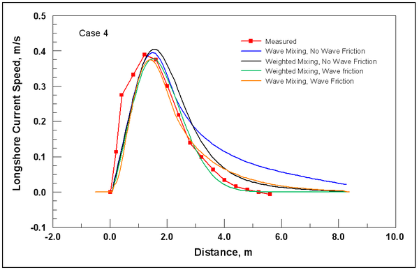
The flux of momentum into the water column from the wind is specified as a function of the wind speed and wind-stress coefficient. Anemometer height above the water or land surface must be considered for accurate estimation of the wind-stress coefficient because wind speed varies logarithmically in the vertical direction for unstratified atmospheric conditions. A general law for the vertical wind profile is given by (Charnock 1955; Hsu 1988):
| (29) |
where
= wind speed at height Z above the surface
= surface roughness
= friction velocity
= von Kármán constant
The friction velocity is defined in terms of the surface wind stress as (Hsu 1988):
| (30) |
where Km = eddy viscosity coefficient, and z is the vertical dimension.
Under the assumption of nearly neutral atmospheric stability, the wind-stress coefficient over water at a height 10 m above the water surface, C10, can be expressed as (Hsu 1988):
| (31) |
where W10 = wind speed in meters per second at 10 m above the surface. Equation 31 includes the assumption of fully developed seas. For measurements of wind speed made at heights other than 10 m, an approximation for the 10-m wind speed is (Shore Protection Manual 1984):
| (32) |
The surface wind-stress Equations 15 and 16, as implemented in CMS-M2D, apply the 10-m wind-drag coefficient and wind speed to compute the surface stress. Thus, values of C10 and W10 defined by Equations 31 and 32 are specified as Cd and W in Equations 15 and 16.
Equations 31 and 32 have been successfully applied in modeling studies investigating motion in strong wind-forced shallow embayments with typical depths ranging from 1 to 4 m (Brown, Militello, and Kraus 1995a; Kraus and Militello 1999; Militello 2000). Calculated water level and current compared well with measurements, indicating that these formulations are satisfactory for estimation of the vertical wind profile and wind stress in shallow-water systems.
Governing Equations for Sediment Motion and Methods for Morphologic Constraints
As a user-specified option, CMS-M2D calculates sediment transport rates and resultant changes in water depth (bottom elevation) through gradients in the transport rates. In CMS-M2D Version 3, three transport rate formulations are available:
- Watanabe (1987) total load formulation.
- Lund-CIRP (Camenen and Larson 2005, 2006) total load formulation (combined suspended and bed load).
- Advection-diffusion (AD) transport for suspended load coupled with either the van Rijn (1998) or the Lund-CIRP formulation for bed load. The AD equation applies the reference concentration and sediment diffusivity from either the van Rijn or Lund-CIRP formulation as a user option.
The sediment transport formulas are applicable with or without the presence of waves. Change in bottom elevation is calculated by the sediment continuity equation in which transport rates computed from a specified formulation are entered. The Lund-CIRP formulas have the properties of smooth transitions between areas of breaking and non-breaking waves and between areas of transport by current only and by a current and waves.
CMS-M2D accounts for the two morphologic constraints of: (a) hard bottom (non-erodible substrate) and (b) bottom avalanching if the slope exceeds a specified value. The approach taken to treat hard bottom allows for sand to accumulate over the hard bottom if depositional conditions are present, and it also allows material overlying the hard substrate to erode while preserving sediment volume. Avalanching is invoked if the bottom slope between two cells exceeds a specified critical slope. The avalanching algorithm applies an iterative approach to move material down slope until the critical slope is no longer exceeded, while conserving sediment volume.
The transport rate formulas that can be applied in CMS-M2D Version 3 are based on the shear stress concept, implying that bed roughness and resulting friction factors are key parameters to estimate when computing transport rates. A sediment transport formula is often developed (i.e., calibrated against data) based on specific equations for calculating bed roughness and associated shear stress. Thus, when calculating the transport rate in CMS-M2D with the three implemented formulas, slightly different approaches are taken to determine the shear stress. In the following sections, the methods are discussed for obtaining the shear stress for each of the sediment transport formulas. Also, it is noted that the roughness and associated shear stresses within the sediment transport calculations are different from those in the CMS-M2D hydrodynamic calculations. The computed current field and properties of surface waves calculated from a separate model are input to the roughness and shear stress calculations for the sediment transport, but there is presently no feedback of roughness or shear stress from the sediment transport component of the model to the hydrodynamic or wave calculations.
CMS-M2D calculates the current velocity in two horizontal coordinate directions (u, v). If there is negligible contribution from the waves to the transporting velocity (e.g., sinusoidal waves), the net transport is in the direction of the resulting current vector and has magnitude of . Thus, waves will contribute to the mobilization and stirring of sediment, but a mean current is needed to produce a net transport. The Watanabe total load formulation and the AD equation compute sediment transport rates along the x and y axes. The Lund-CIRP total load formula computes transport in the direction of the current. In order to obtain the Lund-CIRP calculated transport in the two horizontal coordinate directions, the transport vector is split up into x- and y-directed components.
The following sections describe the sediment transport equations applied in CMS-M2D, followed by the methodologies implemented to treat hard bottom and avalanching.
Watanabe Formulation
The total load sediment transport rate of Watanabe (1987) is given by:
| (33) |
where
= total load (both suspended and bed load)
= maximum shear stress at the bed
= shear stress at incipient sediment motion
= depth averaged current velocity
= density of water
= acceleration of gravity
= empirical coefficient typically ranging from 0.1 to 2
The shear stress at incipient motion is:
| (34) |
where
= sediment density
= median grain diameter
= critical Shields parameter
For the case of currents only (no waves) the bed shear stress is:
| (35) |
where is the current friction factor and in Equation 33. The current friction factor is given as (van Rijn 1998):
| (36) |
in which = total depth defined as , and = Nikuradse equivalent sand grain roughness obtained from:
| (37) |
If waves are present, the maximum bed shear stress is given by a data-based method of (Soulsby 1997):
| (38) |
where = mean shear stress by waves and current over a wave cycle,
= wave bed shear stress, and = angle between the waves and the current. The mean wave and current shear stress is:
| (39) |
The wave bed shear stress is given by:
| (40) |
where = the wave friction factor, and = wave orbital velocity amplitude.
The wave friction factor is (Nielsen 1992):
| (41) |
where is the relative roughness defined as:
| (42) |
where is the semi-orbital excursion defined as:
| (43) |
Transport rates are set to zero at the beginning of the simulation, then updated at each sediment transport time step.
Lund-CIRP Formulation
The Lund-CIRP formulation is implemented into CMS-M2D in two modes. One mode is calculation of total load through combining bed load and suspended load transport. The second mode is implementation in the AD transport equation. Bed roughness and friction factors applied in the Lund-CIRP formulation are first introduced, followed by descriptions of the bed load and suspended load formulations, respectively.
Bed roughness and friction factors
Bottom roughness ks is assumed to consist of three components, namely grain related roughness ksd, form-drag roughness ksf, and sediment-related roughness kss (Soulsby 1997). Total roughness is obtained as the linear sum of these components:
| (44) |
where the grain-related roughness is given by Equation 37. Form-drag roughness is primarily a function of the ripple properties and calculated as (Soulsby 1997):
| (45) |
in which Hr = ripple height, and Lr = ripple length, which are computed from:
| (46) |
for a current (Soulsby 1997) and from:
| (47) |
for waves (van Rijn 1993), where ![]() = mobility parameter that is defined by:
= mobility parameter that is defined by:
| (48) |
and s = specific density given by:
| (49) |
The sediment-related roughness is given by Wilson (1966, 1989):
| ( SEQ Ch4Eq \* MERGEFORMAT 50) |
where ![]() = Shields parameter for current or waves (i = c, w, respectively, for current and waves). Expressions for the Shields parameter for currents
= Shields parameter for current or waves (i = c, w, respectively, for current and waves). Expressions for the Shields parameter for currents![]() and for waves
and for waves![]() are given by:
are given by:
| (51) | |
| (52) |
Equation 50 has to be solved simultaneously with the expression for the shear stress, because the roughness depends on the stress. Explicit predictive equations were developed using approximating polynomials to the exact solution avoid time-consuming iteration in calculating the shear stress. Based on the roughness estimate, friction factors for current fc and waves fw are separately computed according to Soulsby (1997) and Swart (1974), respectively as:
| (53) | |

|
(54) |
where ![]() =Von Karman constant (taken to be 0.4). Shear stress from the current is given by:
=Von Karman constant (taken to be 0.4). Shear stress from the current is given by:
| (55) |
whereas the maximum shear stress from the waves is estimated from:
| (56) |
and the mean shear stress is obtained from:
| (57) |
where a sinusoidal wave is assumed. The corresponding shear velocities for current and waves, respectively, are defined as:
| (58) |
for the current, and:
| (59) |
for the waves (based on the maximum shear stress).
Bed load
A general transport formula for bed load
![]() under combined waves and current was developed by Camenen and Larson (2005):
under combined waves and current was developed by Camenen and Larson (2005):
| (60) |
where subscripts w and n refer to the wave direction and the direction normal to the waves, respectively, a and b are coefficients, and
![]() and
and
![]() are the mean and maximum Shields parameter for waves and current combined, respectively, not including the bed form roughness. The coefficient an = 12 for the transport component normal to the wave direction (current-driven transport). The coefficient b describes initiation of motion and is specified as b = 4.5.
The quantities
are the mean and maximum Shields parameter for waves and current combined, respectively, not including the bed form roughness. The coefficient an = 12 for the transport component normal to the wave direction (current-driven transport). The coefficient b describes initiation of motion and is specified as b = 4.5.
The quantities
![]() and
and
![]() represent the net contribution of the shear stress to the transporting velocity during a wave cycle in the direction parallel and normal to the waves, respectively, defined as:
represent the net contribution of the shear stress to the transporting velocity during a wave cycle in the direction parallel and normal to the waves, respectively, defined as:
| (61) |
in which:
| (62) |
and
| (63) |
where Twc = period of positive flow, Twt = period of negative flow, and uw = time-varying horizontal bottom orbital velocity ( ). Analytical solutions to these equations are available for simple expressions of uw. The friction factor for combined wave and current flow is calculated from Madsen and Grant (1976):
| (64) |
where
![]() and fc and fw are the friction coefficients for current only and waves only, respectively, not including the bed form roughness. The Shields parameter that determines the amount of sediment mobilized for transport is obtained as:
and fc and fw are the friction coefficients for current only and waves only, respectively, not including the bed form roughness. The Shields parameter that determines the amount of sediment mobilized for transport is obtained as:
| (65) |
and the Shields parameter applied in the initiation of motion term is:
| (66) |
where
![]() and
and
![]() are the Shields parameters for current only and waves only, respectively, and the index m denotes the mean value. For sinusoidal waves,
are the Shields parameters for current only and waves only, respectively, and the index m denotes the mean value. For sinusoidal waves,
![]() .
Values of the transport rate coefficients were obtained through calibration against a large data set from laboratory and field experiments involving a mean current, oscillatory waves (sinusoidal and asymmetric), and combined waves and current. A wide range of current and wave velocities, grain sizes, and roughness conditions were covered in this combined data set. The following relationship was developed for the transport coefficient in the wave direction (Camenen and Larson 2005):
.
Values of the transport rate coefficients were obtained through calibration against a large data set from laboratory and field experiments involving a mean current, oscillatory waves (sinusoidal and asymmetric), and combined waves and current. A wide range of current and wave velocities, grain sizes, and roughness conditions were covered in this combined data set. The following relationship was developed for the transport coefficient in the wave direction (Camenen and Larson 2005):
| (67) |
In many applications, the waves are assumed to be sinusoidal, having no asymmetry. Thus, the contribution to the transporting velocity from the waves is negligible, implying that only the current moves the material. Waves are still important for mobilization of the sediment. For such conditions, Equation 60 simplifies to:
| (68) |
where the transport qbc is obtained in the direction of the current, and the transport normal to the current is zero. (There is no velocity component to move the material in this direction.)
Suspended load
The suspended load qs is calculated based on the assumptions of an exponential concentration profile and a constant velocity over the water column to yield (Camenen and Larson 2006):

|
(69) |
where wf = sediment fall speed, cR = reference concentration, and![]() = sediment diffusivity (or mixing coefficient). The transport qs is taken to be in the direction of the current because the waves are assumed to produce a zero net drift and not contribute to the transport. In the calculation of cR and
= sediment diffusivity (or mixing coefficient). The transport qs is taken to be in the direction of the current because the waves are assumed to produce a zero net drift and not contribute to the transport. In the calculation of cR and![]() , the total shear stress should be applied, including the bed form roughness. The reference concentration is given by:
, the total shear stress should be applied, including the bed form roughness. The reference concentration is given by:

|
(70) |
where the coefficient![]() is determined by the following relationship:
is determined by the following relationship:
| (71) |
and the dimensionless grain size is defined by![]()
. The sediment diffusivity is related to the energy dissipation according a generalization of the treatment of Battjes (1975):

|
(72) |
where De is a total effective dissipation given by:
| (73) |
in which kc, kw, and kb are coefficients. The dissipations from bottom friction due to current Dec and from bottom friction due to waves Dew are expressed as:
| (74) | |
| (75) |
and the dissipation due to wave breaking Deb is directly provided from a wave transformation model (e.g., STWAVE. WABED). The coefficient kb corresponds to an efficiency factor and was found to be 0.017, whereas kc and kw are related to the Schmidt number that expresses the ratio between diffusivity of sediment and water (i.e., momentum). These two coefficients are given by:

|
(76) |
where![]() = Schmidt number and the subscript i = c or w denotes current and waves, respectively. The Schmidt number is calculated from the empirical relationships:
= Schmidt number and the subscript i = c or w denotes current and waves, respectively. The Schmidt number is calculated from the empirical relationships:
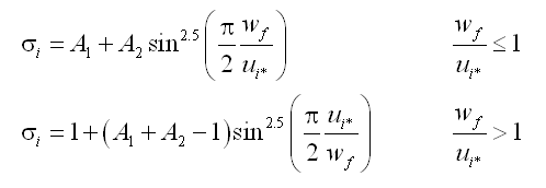
|
(77) |
where A1 = 0.7 and A2 = 3.6 for current, and A1 = 0.09 and A2 = 1.4 for waves. In the case of coexistent waves and current, a weighted Schmidt number is applied according to:
| (78) |
for both waves and current.
Bed load and suspended load transport rates are set to zero at the beginning of the simulation, then updated at each sediment transport time step.
Advection-Diffusion Equation
Calculations of suspended load and bed load are conducted separately through solution of the AD equation for suspended load. This method calculates the suspended load in the water column through the lateral and vertical movement of the sediment.
Basic equations
Sediment transport consists of two components, bed load and suspended load. The bed load and suspended load transport rate formulas are based on the local shear stress. However, in the situation where the suspended sediment concentration rapidly changes in time and space, such as at a river mouth, inlet entrance, navigation channel, and in the vicinity of structures, the suspended load cannot be determined solely by the local forcing conditions. In this case, suspended sediment concentration is governed by the AD equation.
The AD equation implemented in CMS-M2D is obtained from the continuity of depth-averaged suspended sediment transport (Figure 2) as:

|
(79) |
in which
The suspended sediment concentration can be solved from Equation 79 at a sediment transport time step.
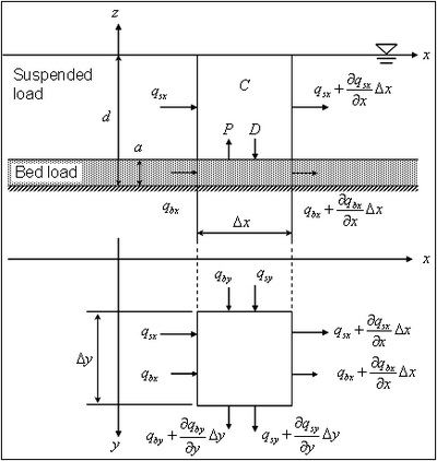
Bed level change is obtained from the sediment continuity equation:

|
(80) |
where qbx = bed load transport rate parallel to the x-axis, qby = bed load transport rate parallel to the y-axis, and p = porosity of sediment.
In Equation 80, the terms
![]() include the bed load component, and the term P-D corresponds to the suspended load component. Figure 2 shows the definition of sediment continuity in a water column, where qsx and qsy are the suspended transport rate in the x and y directions, respectively, and a is the height of the bed load layer. The transport rates qsx and qsy may be defined as follows from Equation 79:
include the bed load component, and the term P-D corresponds to the suspended load component. Figure 2 shows the definition of sediment continuity in a water column, where qsx and qsy are the suspended transport rate in the x and y directions, respectively, and a is the height of the bed load layer. The transport rates qsx and qsy may be defined as follows from Equation 79:

|
(81) |

|
(82) |
Sediment concentration and bed load and suspended load transport rates are set to zero at the beginning of the simulation, then updated at each sediment transport time step.
Pick-up and deposition rates
The AD model calculates the bed level change due to suspended load from the difference between pick-up rate and deposition rate in Equation 80. The pick-up rate and the deposition rate are also applied as the bottom boundary condition in Equation 79. The boundary conditions are specified at an arbitrary level a above the mean bed level:

|
(83) |
| (84) |
where c = equilibrium concentration of suspended sediment at a given elevation, and z = vertical coordinate. Both ca and c0 are reference concentrations defined at z = a. Because the upward flux of sediment depends on the bed shear stress, ca is determined from the bed shear stress calculated from the local hydrodynamic conditions. Representation of ca within CMS-M2D is dependent on selection of either the van Rijn or Lund-CIRP models. The downward sediment flux depends on the concentration in the upper water column; therefore, c0 is specified from solution of Equation 79.
Assuming that the suspended concentration is in equilibrium
![]() , then the basic equation for suspended sediment concentration can be written:
, then the basic equation for suspended sediment concentration can be written:

|
(85) |
This equation can be solved analytically by applying an appropriate mixing coefficient
![]() , and the vertical profile of suspended concentration is obtained in the following form:
, and the vertical profile of suspended concentration is obtained in the following form:
| (86) |
where F(z) is a function of the vertical concentration distribution. The relationship between the reference concentration c0 and the depth-averaged concentration C is:
| (87) |
Thus, c0 may be written in the following form by introducing a conversion function d:

|
(88) |
The bed level change due to suspended load is based upon the difference of the two types of reference concentration:
| (89) |
This equation implies that erosion occurs if ca > c0, and accretion occurs if ca < c0.
In the AD model, three methods of specifying ca and c0 (that is,
![]() )are implemented. Two of the methods are based on the van Rijn formula (van Rijn 1985) and one on the Lund-CIRP formula (Camenen and Larson 2006). Table 1 summarizes general features of the methods.
)are implemented. Two of the methods are based on the van Rijn formula (van Rijn 1985) and one on the Lund-CIRP formula (Camenen and Larson 2006). Table 1 summarizes general features of the methods.
van Rijn formula
The reference concentration ca in the van Rijn formula is given by:

|
(90) |
where a = reference height and
![]() s,max = maximum bed shear stress given by Equation 38.
s,max = maximum bed shear stress given by Equation 38.
| Features of Calculation of Pick-up and Deposition Rates | |||
| Method | Reference Concentration | Conversion Parameter | Comments |
| Exponential Profile | Eq. 90 | Eq. 104 and 105 | Fast computation. Tends to overestimate sediment transport rate. Can be used for some tests. |
| Van Rijn Profile | Eq. 90 | Solves Eq. 85 numerically with Eq. 103 (Runge-Kutta 4th) | Requires substantial computing time. Provides the same results as van Rijn (1985). |
| Lund-CIRP Profile | Eq. 70 | Eq. 104 and 72 | Fast computation. Newly developed sediment transport formula. |
The current-related shear stress is calculated from:

|
(91) |
The wave-related shear stress is given as:
| (92) | |
| (93) |
where = roughness height defined as:
| (94) |
in which ksd and kss are calculated from Equations 37 and 50, respectively.
Bed concentration in the van Rijn model is defined at the height a as:
| (95) |
where Hr = ripple height. If ripples are present, the total roughness height is modified as:
| (96) |
where, ksf = 20(Hr2/Lr) is specified for the van Rijn formula, and ksf = 7.5(Hr2/Lr) is specified for the Lund-CIRP formula. The ripple dimension is obtained by selecting the largest ripple height for the case of current or waves (Equations 46 and 47).
The conversion parameter ![]() to determine c0 is obtained from the vertical mixing coefficient. Van Rijn (1985) proposed a distribution of the mixing coefficients for only current or waves according to Figure 3. The current-related mixing coefficient is given by:
to determine c0 is obtained from the vertical mixing coefficient. Van Rijn (1985) proposed a distribution of the mixing coefficients for only current or waves according to Figure 3. The current-related mixing coefficient is given by:
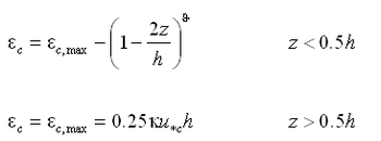
|
(97) |
where u*c = current-related bed shear velocity expressed as:

|
(98) |
and![]() is a coefficient obtained from:
is a coefficient obtained from:
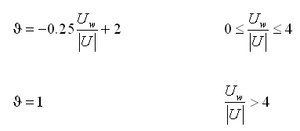
|
(99) |
Figure3. Vertical distributions of mixing coefficient due to current and waves
The wave-related mixing coefficient is:
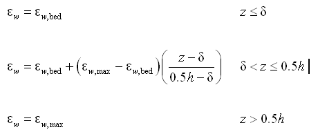
|
(100) |
where

|
(101) |

|
(102) |
in which the parameter = height from the bed given by
, H = significant wave height, and T = significant wave period. If waves and current coexist, the combined mixing coefficient is given by:
| (103) |
By applying the expression for ![]() cw, the concentration profile can be derived from Equation 85, and the conversion parameter
cw, the concentration profile can be derived from Equation 85, and the conversion parameter![]() calculated. In the AD-model based on the van Rijn equations, two methods are implemented to calculate
calculated. In the AD-model based on the van Rijn equations, two methods are implemented to calculate
![]() . One is based on an exponential profile employing a depth-averaged mixing coefficient
. One is based on an exponential profile employing a depth-averaged mixing coefficient![]() , and the other uses the original van Rijn profile, where the
, and the other uses the original van Rijn profile, where the ![]() is obtained by numerical integration of Equation 85. Assuming an exponential profile of suspended sediment concentration,
is obtained by numerical integration of Equation 85. Assuming an exponential profile of suspended sediment concentration,![]() is obtained analytically as:
is obtained analytically as:
| (104) |
where

|
(105) |
Lund-CIRP formula
Reference concentration and sediment diffusivity calculated by the Lund-CIRP formula may also be applied in the AD-model. The formulas used for cR and ε are presented in the section describing the Lund-CIRP formula.
Horizontal diffusion coefficient
Horizontal diffusion coefficients Kx and Ky for the depth-averaged sediment concentration in the AD equation are calculated by the equation proposed by Elder (1959):

|
(106) |
In the surf zone, waves contribute significantly to lateral mixing, and the eddy viscosity coefficient is expected to be a function of the wave properties. For the horizontal diffusion coefficients for AD equation, surf zone mixing proposed by Kraus and Larson (1991) is applied as well as for hydrodynamic calculation.
| (107) |
where![]() describes the lateral mixing below trough level (Smith, Larson, and Kraus, 1993) and is expressed as (Kraus and Larson 1991):
describes the lateral mixing below trough level (Smith, Larson, and Kraus, 1993) and is expressed as (Kraus and Larson 1991):
| (108) |
where ![]() = empirical coefficient representing the lateral mixing strength.
= empirical coefficient representing the lateral mixing strength.
The transition between surf zone diffusion and oceanic diffusion seaward of the breakpoint is represented in CMS-M2D by a weighted mixing coefficient specified as:

|
(109) |
where the weighting parameter![]() is given by:
is given by:

|
(110) |
Bed load transport rate
Bed load transport rate may be calculated with the van Rijn (1998) or Lund-CIRP (Camenen and Larson 2005) formula. In the van Rijn formula, bed load transport rate is obtained from, not including bed roughness:

|
(111) |
The Lund-CIRP formula for bed load is described previously in this chapter.
Scaling Factors for Bed Load and Suspended Load Transport Rates
Adjustments to the bed load and suspended load transport rates can be assigned for both the Lund-CIRP total load formulation and the AD equation. Scaling factors are applied directly to transport rate values as coefficients independently for the bed load transport rate and for the suspended load transport rate. Thus, the bed load transport rate can be scaled separately from the suspended load transport rate. Recommended ranges for the scaling factors are 0.1 to 4. A scaling factor of 1 will not modify the transport rate, and this value is the default. Values less than 1 will reduce the transport rate, and values greater than 1 will increase it. Scaling factors are sometimes found necessary because of uncertainties in forcing and initial conditions, allowing adjustment of model predictions of sediment transport rates and morphology change to observations.
Sediment Continuity Equation
Depth change for the total load formulations and for bed load transport from the AD equation is calculated by the sediment continuity equation, in which time-averaged transport rates are applied. This approach requires that two time intervals be defined, one over which to compute instantaneous transport rates dtsed and the other over which to compute averaged transport rates and morphology change dtmorph. Directional instantaneous transport rates ![]() and
and![]() are calculated at intervals of dtsed and averaged over the time interval dtmorph to obtain the time-averaged transport rates
are calculated at intervals of dtsed and averaged over the time interval dtmorph to obtain the time-averaged transport rates ![]() and
and
![]() for the x and y directions, respectively. Enhancement of down-slope transport and reduction of up-slope transport rates is accomplished by calculation of modified time-averaged transport rates
for the x and y directions, respectively. Enhancement of down-slope transport and reduction of up-slope transport rates is accomplished by calculation of modified time-averaged transport rates
![]() and
and ![]() as (Watanabe 1987):
as (Watanabe 1987):
| (112) | |

|
(113) |
in which ![]() = empirical slope coefficient with typical range of 5 to 30, and
= empirical slope coefficient with typical range of 5 to 30, and ![]() is the time-
averaged transport rate. These formulations add an effective diffusion of transport to the continuity equation for bed change.
is the time-
averaged transport rate. These formulations add an effective diffusion of transport to the continuity equation for bed change.
The sediment continuity equation is solved to compute depth change at the time interval dtmorph and for total load formulations is given by:

|
(114) |
At forcing boundaries, the gradient in transport rate across the boundary cell is set to zero.
For the AD-model, the sediment continuity equation is provided by Equation 80. The time intervals to compute instantaneous transport rates and to compute averaged transport rates and morphology change are consistent with those applied in the total load model, that is, dtsed and dtmorph respectively. Also, the bed load components in Equation 80 are modified by the slope effect as:
Where
|
(115) | |

|
(116) |

|
(117) |
which contains both bed load and suspended load components. At forcing boundaries, the gradient intransport rate across the boundary cell is set to zero.
Hard-Bottom Methodology
Representation of hard (non-erodible) substrate provides the capability to simulate mixed bottom types within a single simulation. The default bottom type in CMS-M2D is erodible, meaning that sediment is available to be transported from that area. Areas having hard bottom are specifically designated as such in the model, and the depth of the hard substrate is specified, allowing representation of either exposed or sediment-covered hard bottom. The one-dimensional (1D) hard-bottom calculation approach applied in the GENESIS shoreline change model (Hanson 1989; Hanson and Kraus 1989) to represent the control of seawalls on shoreline evolution (Hanson and Kraus 1985, 1986) was extended to two dimensions and implemented in CMS-M2D (Hanson and Militello 2005).
The presence of hard bottom exerts a constraint on water depth because the bottom cannot erode. Representation of hard bottom applies an adjustment to the potential transport rates (calculated by a transport formulation with no restriction) to account for the presence of hard substrate. Treatment of hard bottom was developed to satisfy the following four properties:
| a. | Areas having hard bottom cannot erode below the level of the hard substrate. |
| b. | Sediment volume is conserved. |
| c. | The direction of sediment transport at a location with hard bottom is the same as that of the direction of potential local transport. |
| d. | Correction to transport rates is always done in the direction of potential sediment transport. If hard bottom is exposed, the reduction in actual transport as compared to the situation without hard bottom is always transmitted to neighboring areas in the direction of transport as governed by the hydrodynamic forcing. |
The general procedure for treating hard bottom is:
| a. | Calculate sediment transport and morphology change without hard-bottom restriction. |
| b. | Assess whether hard-bottom cells have eroded below the hard bottom depth. If so, apply a correction procedure that adjusts transport rates based on available sediment at hard-bottom cells and corrects depths so that the hard-bottom constraint is not violated. The correction procedure makes adjustments at all cells in which transport rates are controlled by hard bottom and can include adjustments at cells that do not have hard bottom. |
The correction procedure involves four steps:
| a. | Identify all cells that have transport at all four faces directed out of the cell, called "Minus4" cells. These Minus4 cells, if they exist, must constitute the first stage of corrections, as they are only ’deliverers’ of sediment to all adjacent cells, not ’recipients’ of material. |
| b. | If the hard bottom is exposed, all transport rates out of the Minus4 cells are reduced. A list of all adjacent cells, with or without hard bottom, that are influenced by exposed hard-bottom cells is generated for later correction to depths and transport rates. |
| c. | Depths at all adjacent cells are then recalculated to account for the reduced influx of sediment. Cells with hard bottom must then be checked for a possible violation of the hard-bottom constraint and corrected as necessary. For each corrected cell, all sediment transport rates out of the cell are in turn corrected, and each of the next generation of affected cells adjacent to it is added to the list of cells to be corrected. Transport rates into a cell are never changed (as it is an outgoing transport from the adjacent cell that is corrected in that cell). |
| d. | After all cells have been checked, the process is repeated to make sure that the hard-bottom constraint is not violated in any cell. |
Corrections to transport rates and depths are based upon the potential transport rate and amount of sand available for erosion. If, after solution of the sediment continuity equation (Equation 114), the updated depth
is greater than the hard-bottom level
, the outgoing transport rates are corrected to match the criterion
. Over one morphologic time step, the total amount of material
, expressed as a vertical quantity that may leave the cell without violating the hard-bottom constraint is:

|
(118)
|
where qin = total influx of sediment from the cell during the morphologic time step. The correction factor K is given as:

|
(119)
|
where qout = total outflux of sediment from the cell during the morphologic time step. To ensure that ![]()
ingoing transport rates are left unchanged, and outgoing transport rates are multiplied by the correction factor K.
A schematic example of the correction procedure is provided for a symmetric computational grid (Figure 4). The domain contains a 9-by-9 grid of calculation cells. Rows (parallel to the x-axis) are numbered 1 through 9, and columns (parallel to the y-axis) are indicated by A through I. Initial bathymetry level is specified to be![]() at all cells, and the hard-bottom level is at
at all cells, and the hard-bottom level is at ![]() (units) at all cells (z is positive downwards from the original bottom level at
(units) at all cells (z is positive downwards from the original bottom level at![]() )
)
Arrows across the cell walls indicate the initial (potential) transport rates. These are of three different magnitudes: 2 units/m/s (black arrows), 5 units/m/s (blue arrows), and 12 units/m/s (green arrows). For demonstration purposes we assume that the cell sizes in the x-direction and the y-direction are the same and that a transport rate of 1 unit/m/s during one time step corresponds to a bottom elevation change of 1.
Numbers inside each cell indicate the potential depth change (positive numbers mean erosion) in each cell, which is a measure of the magnitude of the depth change if the hard bottom were not there. Thus, in each cell with a depth change that is greater than 5, the hard bottom is exposed. As a result, the actual depth change is limited to 5. Once this depth is reached, the transport out of the cell is reduced owing to limited sediment availability.
In the model, this reduction is accomplished through a correction procedure. The following section explains how this correction is performed through three successive correction loops in a hierarchical and systematic order.
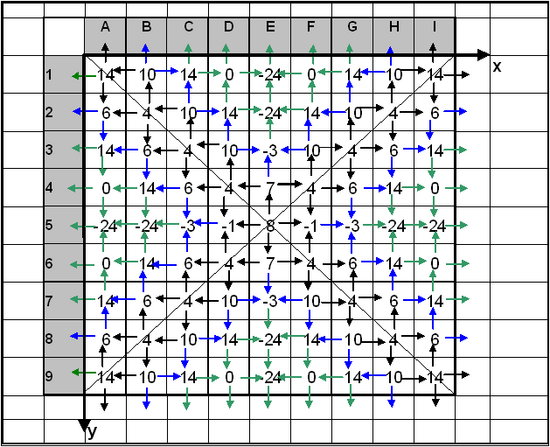
Figure4. Schematic hard-bottom grid and potential transport rates
Correction loop 1:
| a. | Find cells with transport rates directed out of the cell through all four faces. These cells represent the ultimate starting points. Cell E5 is the only cell in this example having outward-directed transport rates through all four faces.
|
| b. | Calculate the new bottom level equaling 8 units, which means that the hard bottom at 5 units is exposed.
|
| c. | Reduce all transport rates out of cell E5 in proportion to the sediment deficit. The potential loss of sediment was 8 units while the available volume in cell E5 was 5 units. Thus, the outgoing transport rates will be reduced from 2 to 2 x 5/8 = 1.25 units/m/s.
|
| d. | Recalculate depths of all adjacent cells, D5, E4, F5, and E6, based on modified transport rates.
|
| e. | Hard bottom is now exposed in cells E4 and E6.
|
| f. | Reduce transport rates out of these two cells (E4 and E6).
|
| g. | Recalculate depths of cells adjacent to E4 and E6 that receive sediment. These cells are D4, E3, F4 and D6, F6, E7. No additional hard-bottom cells are exposed. Thus, the deficit associated with cell E5 does not spread further.
|
Correction loop 2:
| h. | Find start cells from where sand-deficit might spread by searching through the grid from one end to the other. Start cells are those that are located on a hard bottom, but do not receive sediment from any other hard-bottom cell.
|
| i. | Find exposed cells (defined as cells where the hard bottom is exposed) and identify by flag IEXP = 1. Start the search in cell A1. This cell is exposed, but sediment is coming in from B1 that is also exposed. The direction of influence will be in the direction of transport, i.e., from B1 to A1. Thus, A1 cannot be a start cell.
|
| j. | Next, proceed to cell A2. This cell is exposed but, as above, it is receiving sediment from cell A1, which is also exposed. Thus, cell A2 is not a start cell.
|
| k. | The same situation prevails for all cells in the A column. Thus, no cells in the A column are start cells.
|
| l. | Next, proceed to cell B1. This cell is exposed. It is only getting sand from B2, but that cell is not exposed, so no correction can come from there. Thus, cell B1 is a start cell.
|
| m. | All remaining cells are checked the same way, and all start cells are added as necessary to the list of cells to be corrected (here referred to as the correction list).
|
| n. | Correct the first cell in the correction list, cell B1. Add adjacent cells receiving sediment from B1 to the correction list, i.e., cells A1 and C1.
|
| o. | Proceed through all start cells, correct outgoing transport rates, and add to the correction list all cells receiving sediment from the start cells.
|
Correction loop 3:
| p. | The next step is to examine all cells connected to start cells. Transport rates need to be corrected if hard bottom is exposed. Adjacent cells receiving sediment are added to the correction list at the next level of correction cells.
|
Through this procedure, cells will always be corrected in a hierarchic order in which all cells of one level are corrected before proceeding to the next level. Corrections are always propagated in the direction of transport without ambiguity regarding which cell affects another. Figure 5 shows the final bathymetry where all (positive) depth changes are less than 5. The figure also shows the transport rates that were unchanged within this correction procedure (indicated by their original colors) together with those transport rates that were changed (indicated by red arrows). It should be noted, however, that the red arrows represent transport rates with very different magnitudes.
Through the correction loops, transport rates modified by the hard-bottom algorithm are not restricted to cells specified as having non-erodible substrate. Adjustments to transport rates take place at hard-bottom and erodable cells and the spatial extent of the modifications is dependent on the spatial influence of the hard bottom under the transport conditions.
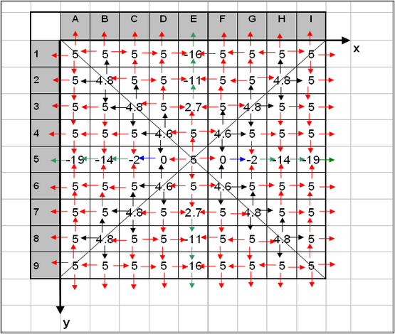
Figure5. Corrected hard-bottom depths and adjusted transport rates
Avalanching Methodology
Controls on bottom slope are implemented through an avalanching algorithm. After each calculation of morphologic change, every cell in the CMS-M2D grid is evaluated to determine if a critical bottom slope has been exceeded. If so, avalanching takes place to reduce the slope. By this method, realistic bathymetric slopes are maintained over the CMS-M2D domain. The method extends an algorithm developed for the Storm-Induced Beach (SBEACH) change model (Larson and Kraus 1989) to two dimensions.
The procedure for determining if avalanching is needed is entered after each calculation of morphologic change. Four slopes are computed for each cell in the grid using the updated depth values. The slopes are computed between each cell and its four neighbors (top, right, bottom, and left neighbors). Starting at the deepest cell in the grid, the bottom slopes are compared to the critical slope, which is the maximum slope allowed before avalanching takes place. If more than one cell has the same depth, cells are checked in order of cell identification number. If the critical slope is exceeded, avalanching takes place with the ending slope being equal to the residual slope after shearing. In the avalanching process, each avalanching calculation includes only the two neighboring cells that exceed the critical slope. Depths of avalanched cells are updated, and the slopes for each of the four neighboring cells recomputed. If more than one slope has exceeded the critical slope, the steepest is avalanched first as it is assumed that it would be the first to reach a critical state. If there is more than one slope that exceeds the critical limit by the same amount, then the slopes are avalanched from north to west in a clockwise fashion.
After an avalanche has occurred, the slopes are recomputed and checked to ensure they have not remained in a critical state. If a critical slope remains, the profile is again avalanched and the process repeated. After all critical slopes have been eliminated, the slopes of all affected cells are recomputed and the algorithm proceeds to the next deepest cell in the grid to repeat the process. All active cells are checked, whether they are wet or dry. After all cells have been checked and, if necessary, avalanched, slopes are again checked against the critical slope. If critical slopes remain, the algorithm finds the deepest cell and the entire process is repeated. If no profiles exceed the critical state, the avalanching process is complete.
A bias can result for cases where there are multiple cells with the same depth or multiple profiles that exceed the critical state by the same degree. In practice, however, it is unlikely that there will repeatedly be multiple cells with equivalent depths or slopes as the values are computed with a high degree of precision.
Numerical Implementation of Governing Equations for Water Motion
Grid definition and discretization of the governing equations are described in this chapter. The governing equations of CMS-M2D are solved numerically on a staggered rectilinear grid by a finite-volume calculation approach. All spatial derivatives are approximated with central differences with the exception of the advection terms, for which an upwind algorithm is applied. The momentum equations are solved first, followed by the continuity equation wherein updated velocity values are applied.
To maximize efficiency of memory for domains with complex shoreline perimeters, the CMS-M2D grid is stored in a 1D array rather than a 2D matrix. The cell numbering convention is described in this chapter. Information is also given on the Courant stability criterion, which provides the user with understanding and an initial approximation of an appropriate model time step for the explicit solution method.
Rectilinear Grid
The governing equations are solved on a discretized domain where cells are defined on a rectilinear grid (which can be regular or irregular), as shown in Figure 6. Each cell has indices i and j that correspond to its position along the x- and y-axes of the grid domain, respectively. Water-surface elevation is calculated at the cell center, whereas the x- and y-components of the velocity are calculated on the left face center and bottom face center of the cell, respectively. Values of flow rate per unit width, qx and qy, are calculated at the same locations as u and v, respectively. Note that the notation for flow rate per unit width is similar to that for sediment transport rate. For the present discussion on hydrodynamics, lower case q denotes flow rate per unit width.
Because the best orientation of the grid may be such that the x- and y-axes do not correspond to geographical coordinates (N-S and E-W), cells in the grid are defined in a local (or grid) coordinate system. The local coordinate system is referenced to geographic coordinates by specification of the angle between the y-axis and true north. A positive value of this angle denotes clockwise rotation and the maximum rotation angle should not exceed 45 deg to retain an orientation as close to geographic as possible.
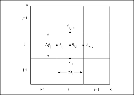
Figure 6. Cell and variable definitions for CMS-M2D
The 2D array format for referencing cell locations is retained here to facilitate presentation of the finite-volume approximations. Mapping of the cell indices from a 2D array to a 1D array is conducted primarily to reduce computer memory requirements. The 1D cell indexing method is discussed below.
Momentum Equations
The finite-volume scheme for the x-momentum equation will be given first, followed by that for the y-momentum equation. Calculation of the bottom stress coefficient, wind stress, eddy viscosity coefficient, and adjustment to the wave stress for shallow water follow the finite-volume approximation of the y-momentum equation because their descriptions are common for both x- and y-momentum equations.
Solution of the momentum equations is conducted to calculate the x- and y-components of velocity u and v, respectively. The explicit approach implemented in CMS-M2D solves each momentum equation for the corresponding flow rate per unit width ![]() or
or ![]() at the present time step k+1 from values calculated at time step k. Velocity components
at the present time step k+1 from values calculated at time step k. Velocity components ![]() and
and ![]() are then calculated from the values of
are then calculated from the values of ![]() and
and ![]() , respectively.
, respectively.
x-momentum equation
The x-momentum equation is solved explicitly by a finite-volume approximation for the control volume shown in Figure 7. The control volume is indicated by the dashed line. Surface and bottom stresses (wind stress and bottom friction) are approximated on the upper and lower surfaces, and momentum fluxes are approximated at each cell face.
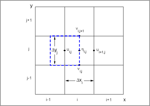
Figure7. Control volume definition for x-momentum equation
The x-momentum equation in finite volume form is given by:
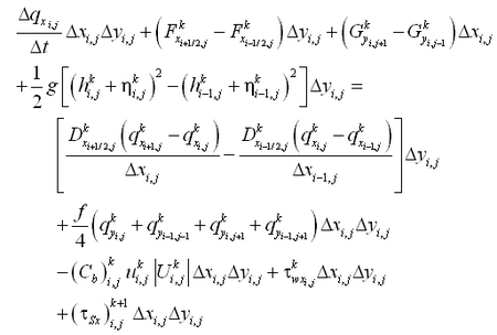
|
(120) |
where
| = | |||
| i, j | = | cell location on the grid | |
| k | = | time step | |
| = | cell-side length parallel to the x-axis | ||
| = | cell-side length parallel to the y-axis |
and
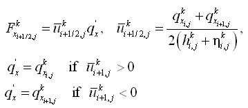
|
(121) |
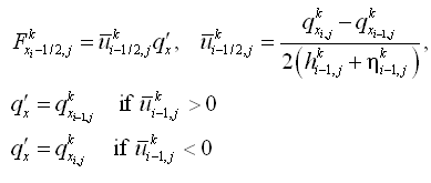
|
(122) |
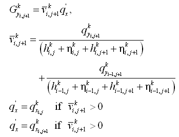
|
(123) |
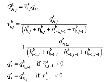
|
(124) |
The x-directed current velocity is given by:

|
(125) |
and the current speed for the x-momentum equation is:

|
(126) |
Wave stress for the x-momentum equation is given by:

|
(127) |
y-momentum equation
The y-momentum equation is solved explicitly with a finite volume approximation for a control volume as shown in Figure 8. The control volume is indicated by the dashed line. Surface and bottom stresses are approximated on the upper and lower surfaces and momentum fluxes are approximated at each cell face.
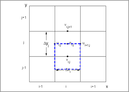
Figure8. Control volume definition for y-momentum equation
The y-momentum equation is finite volume form is given by:
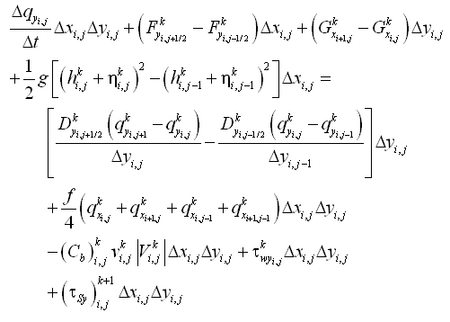
|
(128) |
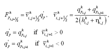
|
(129) |
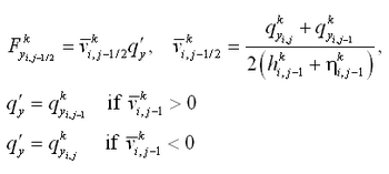
|
(130) |
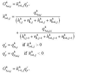
|
(131) |
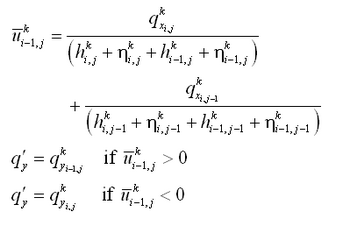
|
(132) |
The y-directed current velocity is given by:

|
(133) |
and the current speed for the y-momentum equation is:

|
(134) |
Wave stress for the y-momentum equation ![]() is given by:
is given by:

|
(135) |
Bottom-friction coefficient
The bottom-friction coefficient ![]() is given by:
is given by:

|
(136) |
where Ci,j = Chezy coefficient calculated as:

|
(137) |
and
if the depth criterion is met. Equation 175 scales the wave stress toward zero as the water depth decreases.
Wave models typically perform calculations in a local right-handed coordinate system in which positive x is directed onshore and positive y is directed alongshore. Thus, the orientation of the local coordinate system may not be aligned with global geographic coordinates. CMS-M2D performs calculations on a local coordinate system that is referenced to global geographic coordinates by the deviation of the y-axis (given in degrees) from true north. If wave stresses are included in CMS-M2D calculations, mapping of those stresses from the wave model to the circulation model must take into consideration the different coordinate systems and grid orientations. Wave stresses calculated by STWAVE or WABED can be automatically mapped to CMS-M2D within the SMS (see Chapter 8).
Continuity Equation
The continuity equation is solved explicitly for water-surface elevation
by a finite-volume approximation for a control volume depicted in Figure 10. Mass fluxes are approximated at each cell face. In the staggered time differencing scheme, the most recently calculated values for the u and v velocity components are entered into the spatial derivatives. The finite-volume approximation of Equation 1 is given by:

|
(176) |
where![]() and all other variables have been previously defined.
and all other variables have been previously defined.
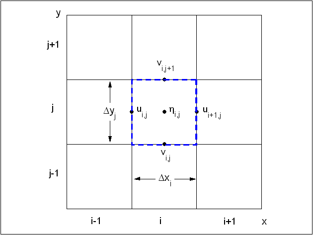
Figure10. Control volume definition for continuity equation
Cell Numbering
CMS-M2D stores its numerical grid in an array rather than a matrix, which saves memory for large or irregular grid domains. The numbering scheme for the computational grid is designed to be efficient such that cells that reside in computationally inactive regions do not have to be stored. For model domains that have complex shorelines, this feature can save substantial computer memory. On the other hand, for simple grids, more memory may be required because pointing arrays are necessary for cell indexing.
The cell numbering system internal to CMS-M2D does not require row and column indexing, but instead assigns each cell a unique identification number. Flather and Heaps (1975) implemented a similar cell numbering system so that only cells included in hydrodynamic calculations were stored. Non-computational regions of the grid, such as the mainland and islands, do not require assigned cell numbers, so they do not occupy space in memory. Figure 11 illustrates the cell numbering system for a small domain that includes a non-computational region indicated by hatching. Cell identification numbers of neighbors adjacent to a particular cell are stored in a pointing matrix within the model. For example, cell 9 has neighbors, with cell identification numbers 12, 10, 4, and 8 moving from top, to right, bottom, and left, respectively. This clockwise order of referencing neighbor cells is taken as convention for descriptions in this document.
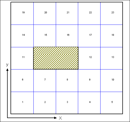
Figure11. Cell numbering system
Locations where no cells exist, such as beyond the computational domain or in non-computational regions such as islands within the domain, are not stored in the grid as cells, but can be referenced as having a cell identification number of 0. For example, cell 11 in Figure 11 lies on the boundary of the grid domain and also resides next to a non-computational area. Neighbor-cell specifications for cell 11 would be stored as 14, 0, 6, and 0. The grid does not contain any cells with a cell number of zero; this value is used in neighbor specification to indicate that a computational cell does not exist at a particular location.
Courant Condition
For an explicit solution method, an initial estimate of the maximum time step for a grid can be calculated from the Courant number x, given by (Richtmyer and Morton 1967):

|
(177) |
The theoretical maximum value of the Courant number is unity for stability of a linear, finite- volume hydrodynamic model, in which for shallow-water equations![]() refers to the speed of a long wave, such as the tide. For a fixed
refers to the speed of a long wave, such as the tide. For a fixed![]() and u, the Courant number limits the value of the hydrodynamic time step
and u, the Courant number limits the value of the hydrodynamic time step![]() .
Because CMS-M2D solves the nonlinear shallow-water equations, stability will be maintained for a Courant number less than unity. Also, for a typical coastal inlet situation, multiple forcing is possible from a superposition of sources other than or in addition to the tide. Contributions to the current can be produced by wind, surface waves, and tributary discharges. Assigning a velocity component to each of these forcings, denoted with a subscript, the Courant number is more accurately defined as:
.
Because CMS-M2D solves the nonlinear shallow-water equations, stability will be maintained for a Courant number less than unity. Also, for a typical coastal inlet situation, multiple forcing is possible from a superposition of sources other than or in addition to the tide. Contributions to the current can be produced by wind, surface waves, and tributary discharges. Assigning a velocity component to each of these forcings, denoted with a subscript, the Courant number is more accurately defined as:
| (178) |
In strong or focused-flow regions of a model domain, such as at ebb shoals and in the surf zone, the wave-driven current can be significantly stronger than the tidal current. Moreover, these are typically areas of greater spatial grid resolution. The combination of strong currents and small grid cells limits the allowable size of the time step in an explicit solution scheme.
Numerical Implementation of Governing Equations for Sediment Motion
Three choices are available for computing sediment transport with CMS-M2D: the Watanabe (1987) formulation, the Lund-CIRP formula (Camenen and Larson 2005, 2006), and the AD equation. The Watanabe transport formula produces a total transport rate, estimating the contributions of combined suspended sediment load and total load in a "calculation-at-a-point" formulation. The Lund-CIRP transport formula computes both bed load and suspended load transport rates, which are combined to obtain a total load transport rate. The AD equation is solved for both suspended load and bed load transport rates.
Morphology change is computed by means of two time steps, a transport rate time step and a morphology change time step. Instantaneous transport rates are computed at the transport rate time step and averaged over the morphology change time step. Averaged transport rates are then applied in the sediment continuity equation. Transport rates calculated by the Watanabe, Lund-CIRP total load formula, and AD equation are instantaneous values.
Watanabe Formulation
Implementation of the Watanabe formulation computes transport rates on cell faces with the x-directed rate![]() located on the left face center and the y-directed rate
located on the left face center and the y-directed rate![]() located on the bottom face center. Thus, for a given cell,
located on the bottom face center. Thus, for a given cell, ![]() and
and![]() are calculated at the same locations as u and v, respectively (Figure 6). Time-averaged face-centered transport rates are applied in the sediment continuity equation to calculated depth change.
are calculated at the same locations as u and v, respectively (Figure 6). Time-averaged face-centered transport rates are applied in the sediment continuity equation to calculated depth change.
Calculation of x- and y-directed transport rates ![]() and
and![]() , respectively, by the Watanabe formulation is conducted in CMS-M2D as:
, respectively, by the Watanabe formulation is conducted in CMS-M2D as:
| (179) | |
| (180) |
The bottom stresses in the situation in which no waves are present are calculated in the x and y directions as:

|
(181) |
and

|
(182) |
in which the velocities and are calculated as:

|
(183) |
and

|
(184) |
The current friction factors for the x and y directions, respectively, are:

|
(185) |
and

|
(186) |
If waves are present, the bottom shear stresses in the x and y directions are calculated as:

|
(187) |
and

|
(188) |
Bottom shear stresses calculated by Equations 187 and 188 are entered as values of![]() and
and ![]() in Equations 179 and 180, respectively.
in Equations 179 and 180, respectively.
Combined wave and current shear stresses for the x and y directions are given by:

|
(189) |
and

|
(190) |
The wave bed shear stresses for the x and y directions, respectively, are given by:

|
(191) |
and

|
(192) |
where the wave friction factor for the x direction is given as:

|
(193) |
and for the y direction is:

|
(194) |
Relative roughness for the x and y directions are given by:

|
(195) |
and

|
(196) |
Wave orbital velocity amplitudes for the x and y directions, respectively, for non-breaking waves are:
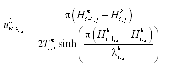
|
(197) |
and
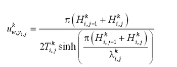
|
(198) |
For breaking waves, the wave orbital velocity amplitudes for the x and y directions, respectively, are:

|
(199) |
and

|
(200) |
Lund-CIRP Formulation
The Lund-CIRP formulation computes sediment transport properties and transport rates at the cell center, which corresponds to the same location in the cell as the water-surface elevation
is calculated (Figure 6). After transport rates are calculated by the Lund-CIRP formulas for all cells in the domain, they are mapped back to the cell faces such that the x-directed rate
is located on the left face center and the y-directed rate
is located on the bottom face center. Time-averaged face-centered transport rates are applied in the sediment continuity equation to calculated depth change.
AD Equation
AD equation for sediment concentration
The AD equation for sediment concentration is solved explicitly for depth-averaged concentration by a finite-volume approximation for a control volume. Depth-averaged concentration C, pick-up rate P, and deposition rate D are approximated at each cell center, and mass fluxes are approximated at each cell face. The finite-volume approximation of Equation 79 is given by:

|
(201) |
where
| = | |||
| = | |||
| i,j | = | cell location on the grid | |
| k | = | time step | |
| = | time step to calculate sediment transport | ||
| = | cell side length parallel to the x-axis | ||
| = | cell side length parallel to the y-axis |
and
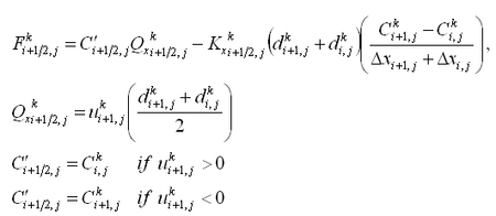
|
(202) |
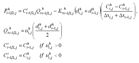
|
(203) |
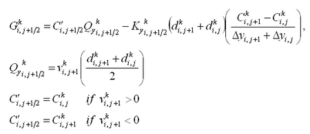
|
(204) |
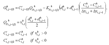
|
(205) |
Pick-up rate and deposition rate
Pick-up rate and deposition rate can be calculated in CMS-M2D by either the van Rijn or Lund-CIRP formulation. The calculation method of P and D for van Rijn formula is described first, then that for Lund-CIRP formula.
Van Rijn model (exponential profile or van Rijn profile)
The pick-up rate P and for van Rijn model is given by:
| (206) | |

|
(207) |
Maximum bottom shear stress ![]() s,max is given by:
s,max is given by:

|
(208) |
where ![]() cs,
cs, ![]() ws, and
ws, and ![]() ms are shear stresses owing to current, wave, and combined wave and current, and are given by:
ms are shear stresses owing to current, wave, and combined wave and current, and are given by:

|
(209) |

|
(210) |

|
(211) |
The current velocity Uc and wave orbital velocity Uw are defined at each cell center.

|
(212) |
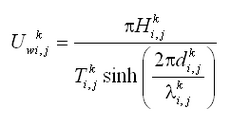
|
(213) |
and wave friction factor is:

|
(214) |
where

|
(215) |
Calculations with CMS-M2D have shown that the van Rijn (1985) reference concentration tends to give an overestimation under strong shear stress, such as in the sheet flow region. Therefore, the following limitation is applied to reduce the overestimate:

|
(216) |
where R is the reduction coefficient expressed as:

|
(217) |
in which cb is the extrapolated bed concentration calculated by Equation 207 with a = d50, which reduces to:

|
(218) |
The deposition rate D for the van Rijn model is given by:

|
(219) |
where βd is the conversion parameter that depends on the user-selected concentration profile. If an exponential profile is selected, βd is calculated by using depth-averaged mixing coefficient ![]() and given by:
and given by:

|
(220) |
and the reference height a is given by:

|
(221) |
where Hr is the ripple height.
If the van Rijn profile is selected, βd has to be calculated numerically because the mixing coefficient varies with height from the bed. In the AD-model with the van Rijn profile, the mixing coefficients are calculated at 20 points in the vertical direction. Mixing coefficients for the current εc and for waves εw are calculated, and then combined as follows:

|
(222) |
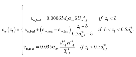
|
(223) |
| (224) |
where

|
(225) |

|
(226) |

|
(227) |
With the mixing coefficient εcw(z) available, the vertical distribution of the concentration c(z) can be solved by the fourth-order Runge-Kutta method. Then, βd values for the van Rijn profile are calculated by numerical integration of the concentration profile:
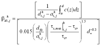
|
(228) |
Lund-CIRP model The pick-up rate P for the Lund-CIRP model is given by:
| (229) |
where ca is the reference concentration given by:

|
(230) |
where AcR = 3.5 10-3exp(-0.3d*), and b = 4.5. Bed shear stresses due to current, wave, and combined current and wave are given by,

|
(231) |

|
(232) |

|
(233) |

|
(234) |
Friction factors for the current and for waves are given, respectively, by:

|
(235) |

|
(236) |
The deposition rate D for the Lund-CIRP model is given by:

|
(237) |
The concentration profile for the Lund-CIRP formula is approximated by an exponential profile. The conversion parameter d is given by:

|
(238) |
where the mixing coefficient ![]() is calculated as:
is calculated as:

|
(239) |
De is the energy dissipation rate owing to current, wave, and wave breaking:
| (240) |
where
| (241) | |
| (242) |
and Db is given from wave model output, and ![]() and
and![]()
Sediment diffusion coefficient
Diffusion coefficients Kx and Ky are defined at cell faces and calculated as:

|
(243) |

|
(244) |

|
(245) |

|
(246) |
Bed load transport rate
Bed load transport rates qbx and qby are calculated at each cell center. For the van Rijn model, they are given by:

|
(247) |

|
(248) |
where

|
(249) |

|
(250) |
Bed load transport rates for the Lund-CIRP model are given by:

|
(251) |

|
(252) |
where an = 12 and b = 4.5.
Boundary conditions
Boundary conditions for the AD equation are given for wall boundary and for open boundary, respectively.
If a cell face is defined as a wall, the suspended load flux on the cell face is set to zero.
| (253) | |
| (254) | |
| (255) | |
| (256) |
For the cell on the open/forcing boundary, the concentration is set as the equilibrium concentration,
| (257) |
where![]() is the depth-averaged concentration on the open boundary cell. Also, the gradient of suspended load flux is setas zero
(
is the depth-averaged concentration on the open boundary cell. Also, the gradient of suspended load flux is setas zero
(![]() )for the open boundary.
)for the open boundary.
| (258) | |
| (259) | |
| (260) | |
| (261) |
Criterion of time step for AD model
Calculation of the AD equation is computed at a time step of Δtsed. To maintain stable calculations in an explicit solution scheme, the following condition must be satisfied:
| (262) |
where Δs is the cell size, and u is the local current speed. During calculation of the AD equation, CMS-M2D evaluates whether this criterion is met. If the criterion is not met, CMS-M2D will reduce Δtsed to maintain stability.
Hard-bottom methodology for AD model
Modification of sediment transport rate owing to hard bottom is also computed in the AD model. Hard bottom is treated separately for suspended and bed load. For suspended load, the methodology assumes that upward sediment flux will be zero if the hard bottom is exposed. The criterion for the maximum pick-up rate is expressed as:

|
(263) |
where hhb is the hard-bottom level, and p is the porosity. For bed load, the methodology of treating hard bottom as described in Chapter 3 is applied.
Sediment Continuity Equation
Calculation of depth change is computed by solution of the sediment continuity equation. Before solving the sediment continuity equation, time-averaged sediment transport rates are computed from the instantaneous transport rate values. Transport rates applied in the sediment continuity calculations are total load transport rates when total load formulations are applied, or bed load transport rates when the AD equation is applied. Thus, for the sediment continuity equation, the subscript t denotes total load for total load formulations and bed load for the AD equation.
Time-averaged transport rates for the x and y directions, respectively, are computed by:

|
(264) |

|
(265) |
in which Nm = number of instantaneous transport rate values, and l = index representing the time at which the instantaneous rates were calculated. Instantaneous rates are calculated at the sediment transport time step![]() , and time-averaged rates apply instantaneous rates averaged over the morphologic change time step
, and time-averaged rates apply instantaneous rates averaged over the morphologic change time step ![]() . Adjustment of the time-averaged transport rate for bottom slope is computed for the x and y directions as:
. Adjustment of the time-averaged transport rate for bottom slope is computed for the x and y directions as:

|
(266) |

|
(267) |
where the total time-averaged transport rates![]() and
and![]() are calculated as:
are calculated as:

|
(268) |
and

|
(269) |
Depth change over the time interval is calculated as:

|
(270) |
Updated depth is then computed by:

|
(271) |
After new depth values are calculated for all cells in the computational domain, they are provided to the hydrodynamic portion of the model so that it can respond to changes in morphology.
For the AD model, calculation of depth change is computed by a method similar to that described above, except that suspended load and bed load components are treated separately. Before solving the sediment continuity equation, time-averaged sediment transport rates are computed from the instantaneous transport rate values. Time-averaged pick-up rate and deposition rate for the suspended load component are computed by:

|
(272) |

|
(273) |
Time-averaged bed load transport rates for the x and y directions, respectively, are computed by:

|
(274) |

|
(275) |
Bed load transport rates for the AD model are defined at each cell center. Solution of the sediment continuity equation requires that the bed load transport rates are defined at the centers of cell faces. Therefore, bed load transport rates are computed on the cell faces by:

|
(276) |

|
(277) |
Further, adjustment of the time-averaged bed load rate for bottom slope is computed for the x and y directions as:

|
(278) |

|
(279) |
Depth change over the time interval is calculated as:

|
(280) |
Updated depth is then computed by Equation 271.
Boundary Conditions
Six types of boundary conditions are implemented in CMS-M2D and are distinguished as specifying a forcing or a non-forcing boundary. Table 2 lists the boundary condition types and contains a short description of each. Each boundary condition type is described next.
| Boundary Condition Types | |
| Boundary Condition | Description |
| Tidal-constituent water-level forcing | Water level specified as sum of tidal constituents |
| Time series water-level forcing | Water level specified from time series input file |
| Time series water-level and velocity forcing | Water level and velocities specified from time series input files |
| Time series flow rate forcing | Flow rate specified from a time series input file |
| Closed, reflective (non-forcing) | Impermeable boundary, velocity must flow parallel to boundary |
| Wave-adjusted water-level and velocity forcing | Boundary water level and velocity values are adjusted for presence of radiation-stress gradients. Provides compatibility of boundary forcing with wave forcing |
Water-Level Forcing Boundary Conditions
Water-level forcing can be specified through either tidal constituents or by time series of water level read from a file. These two boundary conditions apply the same calculation approach, with the distinguishing feature between them being the source of the water level prescribed at the boundary.
If a cell is designated as a water-surface elevation boundary cell, the continuity equation for that cell is not solved, and the water level is updated each time step according to:

|
(281) |
where![]() is a prescribed value. If tidal forcing is specified, then
is a prescribed value. If tidal forcing is specified, then
| (282) |
Tidal-constituent forcing
Tidal-constituent forcing in CMS-M2D can accommodate as many as eight components of the astronomical tide. The user can select from the following constituents: M2, S2, N2, K2, K1, O1, M4, and M6. Although the M4 and M6 constituents are harmonics, they can be generated in continental shelf areas and may be present as components of the tidal forcing at the grid boundary. Specification of tidal constituents requires input information for the local amplitude and phase values. Tidal-constituent forcing by CMS-M2D is simple and does not include advanced tidal calculations or relations to Greenwich tidal parameters (Schureman 1924).
Tidal elevation
is given by:

|
(283) |
where A = amplitude (m), s = speed (deg/hour), and f = phase (deg) of the tidal constituent. Constituents can be eliminated from the tidal forcing by setting their amplitudes to zero. If the tidal elevation boundary condition is invoked, water levels at tidal boundary cells are computed at every time step. Tidal phase and amplitude is held constant across the tidal-constituent boundary. For applications requiring amplitude and phase variation over an open boundary, two approaches to forcing the boundary are available. Time series of tidal curves along the boundary can be developed within the SMS in which the tidal information is obtained from a tidal-constituent database. Alternatively, solutions from regional models can be applied to map water-surface elevations as boundary conditions for CMS-M2D.
Time series water-level forcing
The time series water-level forcing boundary condition is specified by water levels (![]() ) read into the model from an input file. Time increments of the forcing data are not required to be equal to, or in multiple increments of, the model time step. Because the model will usually have a hydrodynamic time step smaller than the time interval between water-level forcing input, CMS-M2D must be instructed on treatment of the water-level boundary value between times that its value is specified in the input file. One option is to linearly interpolate in time between input water-level values, and this is the preferred option. A second option is to keep the water level constant between input water-level values. The boundary condition input file for water level contains a parameter that sets the interpolation option.
) read into the model from an input file. Time increments of the forcing data are not required to be equal to, or in multiple increments of, the model time step. Because the model will usually have a hydrodynamic time step smaller than the time interval between water-level forcing input, CMS-M2D must be instructed on treatment of the water-level boundary value between times that its value is specified in the input file. One option is to linearly interpolate in time between input water-level values, and this is the preferred option. A second option is to keep the water level constant between input water-level values. The boundary condition input file for water level contains a parameter that sets the interpolation option.
Time Series Water-Level and Velocity Forcing Boundary Condition
The time series water-level and velocity forcing boundary condition applies velocities at cell boundaries in addition to water levels. Application of water levels for this boundary type is identical to that previously described for water-level forcing boundary conditions. Velocities prescribed on the boundaries enter the momentum equation through the advective terms. Discretization of the momentum equations for applying velocities on the boundaries is identical to the implementation for non-boundary cells described in Chapter 4.
Time Series Flow Rate Forcing Boundary Condition
The time series flow rate forcing boundary condition can be assigned at locations where the flow rate is known. Typical examples where this boundary condition is applied are natural tributaries (rivers, streams, and creeks), controlled-discharge canals, and anthropogenic intake or discharge locations such as for power plant cooling water or treatment plant outfalls.
A flow rate boundary condition specifies discharge at one or more cells on the grid boundary. If a cell is designated as a flow rate boundary cell, the momentum equation for the appropriate cell face is not solved, and the flow-component normal to the face is prescribed. Because CMS-M2D operates on a staggered grid, virtual cells are added to the right or top of the grid at flow rate forcing boundary cells prescribed on those sides. Addition of virtual cells, where water-surface elevation and current are not calculated, is required to calculate fluxes at cell faces on the right or top of the grid.
For a flow rate forcing cell located on the right side of the grid at location i+1,j, the flux is given by:

|
(284) |
where ![]() = input flow rate directed parallel to the x-axis, and i+1
denotes an imaginary cell adjacent and to the right of the ith cell.
For a flow rate forcing cell located on the left side of the grid at location
= input flow rate directed parallel to the x-axis, and i+1
denotes an imaginary cell adjacent and to the right of the ith cell.
For a flow rate forcing cell located on the left side of the grid at location
i-1,j,the flux is given by:

|
(285) |
For a flow rate forcing cell located on the top side of the grid at location i,j+1,the flux is given by:

|
(286) |
where![]() = input flow rate directed parallel to the y-axis.
= input flow rate directed parallel to the y-axis.
For a flow rate forcing cell located on the bottom side of the grid at location
i,j-1, the flux is given by:

|
(287) |
Closed, Reflective Boundary Condition
The closed, reflective boundary condition is specified at impermeable boundaries, such as at the land-water interface. These boundaries behave as walls; water can flow parallel to the wall face, but not through it.
The normal velocity at a closed boundary on the left cell face is:
| (288) |
and the normal velocity at a closed boundary on the bottom face is:
| (289) |
Closed boundaries on the right and top cell faces are prescribed at the imaginary cells i+1,j and i,j+1, respectively.
Wave-Adjusted Water-Level and Velocity Forcing
Simulations for nearshore areas may have available boundary forcing information that does not include the presence of waves. The wave-adjusted water-level and velocity boundary condition modifies the prescribed forcing values to account for waves. If water-level forcing or mixed water-level and velocity forcing are applied together with radiation-stress forcing, then in this boundary condition, boundary values are adjusted for wave-driven current and set up or set down. Boundary adjustment is conducted by creating a surface deflection (set up and set down) consistent with that of the interior solution so that radiation stress-forced flow can move smoothly through the boundary (Reed and Militello 2005). It is believed that this boundary condition is new to coastal circulation modeling.
Implementation of the wave-adjusted boundary conditions within CMS-M2D is automated. Thus, if radiation-stress gradients are applied as forcing, CMS-M2D will automatically apply the wave-adjusted boundary condition to adjust the prescribed forcing for the presence of waves.
Adjustment to the prescribed boundary conditions is conducted by solving the 1D continuity and momentum equations normal to the boundary, in which the radiation stress gradient is included in the momentum equation. The forms of the 1D continuity and momentum equations for the x-direction are:

|
(290) |

|
(291) |
in which:
| (292) |
where ![]() is the applied boundary condition,
is the applied boundary condition,![]() is the prescribed boundary value (read from a file),
is the prescribed boundary value (read from a file),![]() and
and ![]() are the solutions from Equations 290 and 291, and
are the solutions from Equations 290 and 291, and
![]() is given by:
is given by:
| (293) |
where ![]() and
and ![]() denote face-centered averages that place h and
denote face-centered averages that place h and ![]() at the same position as
at the same position as ![]() . If the boundary is specified a mixed water-surface elevation and velocity boundary, then the u-component of velocity assigned at the boundary is modified by:
. If the boundary is specified a mixed water-surface elevation and velocity boundary, then the u-component of velocity assigned at the boundary is modified by:
| (294) |
where u is the applied velocity at the boundary and ub is the prescribed velocity (read from a file).
The 1D continuity and momentum equations for the y-direction are:

|
(295) |

|
(296) |
where ![]() and
and ![]() are the solutions from Equations 295 and 296, and
are the solutions from Equations 295 and 296, and ![]() is given by:
is given by:
| (297) |
where ![]() and
and ![]() are face-centered averages that place h and
are face-centered averages that place h and ![]() at the same position as
at the same position as
![]() . If the boundary is specified as a mixed water-surface elevation and velocity boundary, then the v component of velocity assigned at the boundary is modified by:
. If the boundary is specified as a mixed water-surface elevation and velocity boundary, then the v component of velocity assigned at the boundary is modified by:
| (298) |
where v is the applied velocity at the boundary and vb is the prescribed velocity (read from a file).
The wave-adjusted boundary condition is demonstrated in Appendix G for an idealized beach.
Model Features
Capabilities have been implemented into CMS-M2D to represent flooding and drying, and other features designed to promote flexibility and convenience of the modeling system. This chapter describes these features and provides information on model options. Topics covered are: flooding and drying, hot-start options, model spin-up, coupling with larger scale circulation models, coupling with wave models, and output options.
Flooding and Drying
Numerical modeling of shallow-water areas such as beaches, flood shoals, or expansive tidal or wind-tidal flats is most accurately performed if realistic and robust flooding and drying algorithms are invoked. Representation of flooding and drying also eliminates the need to modify grid depth to avoid artificially induced instabilities. Numerical simulation of flooding and drying of cells or elements in hydrodynamic models has been performed with various techniques such as application of barrier and weir equations (Reid and Bodine 1968; Butler 1978; Wanstrath 1978) and moving boundaries (Yeh and Chou 1978). A simple and robust flooding and drying algorithm has been implemented to represent inundation and drying of shallow areas of the model domain.
Criteria were established for the flooding and drying algorithms implemented in CMS-M2D and are given in Table 3. The criteria were specified so that the algorithms would produce realistic behavior, and numerical problems, such as oscillations and flutter, would be minimized.
| Criteria for Flooding and Drying Algorithms | |
| Flooding | Comments |
| Water depth must exceed a specified minimum depth | Transfer of physically meaningful water volume, avoids flutter |
| Water must be moving toward dry cell | Takes into account wind-induced set up, avoids instability |
| Drying | Comments |
| Total water depth is less than specified minimum depth | Definition of drying |
Every wet cell is checked to determine whether or not it has dried after new water-level and velocity values have been calculated over the model domain. The criterion for a cell to be dry is:
| (299) |
where ![]() = total water depth, and
= total water depth, and ![]() = depth below which drying is assumed to occur. If a cell or its adjacent neighbor to the south or west has become dry, restrictions on flow between the two cells are imposed. Restrictions governing flow across the two faces are imposed for the following conditions:
= depth below which drying is assumed to occur. If a cell or its adjacent neighbor to the south or west has become dry, restrictions on flow between the two cells are imposed. Restrictions governing flow across the two faces are imposed for the following conditions:
| a.Both cells on each side of a face are dry. | |
| (300) |
| (301) |
This restriction sets the velocity at the face to zero so that there is no transfer of water between dry cells.
| b.Neighbor to south or west is dry, and cell i,j is wet. | |
| (302) | |
| (303) |
This restriction sets the velocity at the face to zero if the velocity at the previous time step indicates transfer of water from a neighboring dry cell to the wet cell i,j. Water is allowed to flow from the wet cell to the neighboring dry cell.
| c.Neighbor to south or west is wet, and cell i,j is dry. | |
| (304) | |
| (305) |
This restriction sets the velocity at the face to zero if the velocity at the previous time step indicates transfer of water from dry cell i,j a neighboring wet cell. Water is allowed to flow from the neighboring wet cell to the dry cell i,j.
Hot-Start Capabilities
CMS-M2D has two hot-start capabilities, and both can be invoked during a simulation. The two hot-start types are:
| a. | Hot-start file written once during a simulation at a user-specified time. The file name prefix is given by the user. This file can be opened in future simulations to initialize CMS-M2D at a convenient time, such as after the model has spun up. | ||||||||||||||||||||||||||||||||||||||||||||||||||||||||||||||||||||||||||||||||||||||||||||||||||||||||||||||||||||||||||||||||||||||||||||||||||||||||||||||||||||||||||||||||||||||||||||||||||||||||||||||||||||||||||||||||||||||||||||||||||||||||||||||||||||||||||||||||||||||||||||||||||||||||||||||||||||||||||||||||||||||||||||||||||||||||||||||||||||||||||||||||||||||||||||||||||||||||||||||||||||||||
| b. | Hot-start file written at user-specified intervals. If this option is invoked, CMS-M2D will alternate hot-start file names HOTSTART1.M2I and HOTSTART2.M2I each time a hot-start file is written. An information file called HOTSTART.INFO is also written that contains the name of the last hot-start file that was written and the simulation time, in hours, when the hot-start file was saved. These hot-start files are helpful in restarting simulations that terminate unexpectedly.
Model Spin-Up: Ramp FunctionModel spin-up is controlled by a hyperbolic tangent function that scales values of the input forcing over a user-specified interval. A time-dependent scaling factor
where Tramp = time over which the model is spun up. All model forcing is multiplied by the scaling factor over the duration of the ramp. After the simulation time exceeds the ramp duration, the scaling factor is set to 1.0. Coupling with Larger-Domain ModelCMS-M2D can be operated as a detailed inset of a larger-domain model. This capability maintains hydrodynamic properties at the CMS-M2D boundaries, increases flexibility in resolution over the project area, and allows for application of options within CMS-M2D that may not be available in other models. Coupling can be invoked by forcing CMS-M2D with water-surface elevations or a combination of water-surface elevations and velocities, where the values have been obtained from a larger-domain model. The SMS provides an automated procedure for extracting and mapping boundary information from a larger-domain model to CMS-M2D (Chapter 8). CMS-M2D can accept boundary information from any larger-domain model, including another CMS-M2D simulation. Considerations for coupling with a larger-domain model are discussed here with an example shown for CMS-M2D forced by water-surface elevations and velocities calculated by ADCIRC. If a larger-domain model is to provide boundary conditions for CMS-M2D, mesh or grid resolution of the larger-domain model in the area of the CMS-M2D boundary must be sufficient to describe details of the hydrodynamic field at the scales required for the particular project. Figure 12 shows a CMS-M2D grid overlaid on a portion of an ADCIRC mesh developed for Shinnecock Inlet, NY. Distances between ADCIRC nodes are a few times larger than the CMS-M2D cell sizes, but are not greatly larger. If the ADCIRC nodes were spaced further apart, having only a few nodes in the vicinity of the CMS-M2D boundary, details of the flow field would not be adequately described to capture the inlet and ocean hydrodynamics of the area. 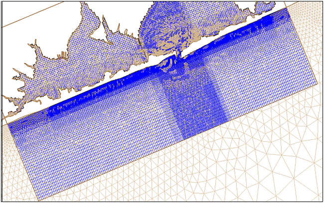 Figure12. CMS-M2D grid and ADCIRC mesh for Shinnecock Inlet, NY Temporal resolution of the boundary information provided to CMS-M2D from the larger-domain model must also be considered. Output frequency of larger-domain model solutions should be set to minimize error in forcing for the scales of motion calculated. As an example, water-level curves calculated by the function , where t is in hours, and output at increments of 1.0 and 0.25 hr are shown in Figure 13. Output at 0.25 hr produces a curve that describes the water level significantly better than the curve output at 1.0 hr. An example of the error introduced by the 1-hr interval output is shown at the second peak, in which a 3-cm difference is encountered. Application of a solution from a regional model as boundary conditions for CMS-M2D can be conducted for simulations in which any combination of tide, wind, and waves are needed. When the regional model is launched, it should contain all forcing to be included in the simulation (tide, wind, etc.) except for waves. Wave forcing should be applied only to the local CMS-M2D simulation. There are two reasons for this approach. First, if waves are applied as forcing, CMS-M2D automatically adjusts its forcing boundaries for the presence of waves (wave-adjusted boundary condition) to compute set up and set down, and to allow wave-driven flow into and out of the domain. If the regional model includes wave forcing, then the regional solution will transmit the wave-driven component of the solution into the CMS-M2D boundary conditions. Combination of the prescribed boundary conditions from the regional model and the wave-adjusted boundary condition will then result in the wave forcing being applied twice at the CMS-M2D boundary. Secondly, the regional model will usually have coarser resolution than the CMS-M2D local grid, and will not have adequate resolution in the surf zone to accurately describe the distribution of set up, set down, and wave-driven currents. If waves are included in the regional model forcing, the interpolation or extrapolation of the wave-driven component of the regional solution to the local CMS-M2D boundary will not contain sufficient detail to accurately describe the response in and near the surf zone. Thus, error will be introduced into the CMS-M2D boundary conditions. 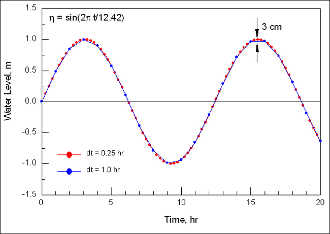 Figure13. Time discretization of a sinusoidal water-level curve Coupling with STWAVE and WABEDCMS-M2D and a wave model such as STWAVE (Militello and Zundel 2003) or WABED (Lin et al. 2006) can be coupled through the SMS Steering Module (Chapter 8). Coupling can be conducted by supplying CMS-M2D with radiation-stress gradients and wave properties calculated by the wave model and by applying currents and water depth (h + η) calculated by CMS-M2D as input to the wave model. The user has the option of selecting one or more of these linkages. Guidance is provided here to assist the user in setting up a correct and successful coupled simulation. CMS-M2D and STWAVE (or WABED) calculate on different coordinate systems that may or may not be aligned, depending on the orientation of the shoreline relative to geographic coordinates. The coordinate system for CMS-M2D can be specified in the range of ± 45 deg from geographic coordinates, meaning, that positive x is directed within 45 deg of east and positive y is directed within 45 deg of north. An angle provided in the CMS-M2D control file defines the deviation of the CMS-M2D grid from geographic coordinates. STWAVE operates on a grid aligned such that the x-axis is directed onshore and the y-axis is directed alongshore. Figure 14 shows three examples of CMS-M2D and STWAVE coordinates for different shoreline orientations. Each model must be independently established so that its coordinate system is consistent with its computational approach. For coupling, the CMS-M2D and STWAVE grids overlap and information is mapped from one model to the other. The SMS automatically calculates any required rotations of components when mapping fields between STWAVE and CMS-M2D. In areas of the computational domain where wave breaking or strong wave-current interaction takes place, resolution for CMS-M2D and STWAVE should be similar. By specifying cells in both models to have similar spacing, coupling efficiency is maximized because high-resolution details calculated by one model are not lost when the solution field is mapped to the other model. Figure 15 shows STWAVE and CMS-M2D grid spacing in the nearshore area. Surf zone width is indicated by the line denoting 10 STWAVE cells. In this area, CMS-M2D and STWAVE have similar spacing in the cross-shore. Cell sizes in the CMS-M2D grid become larger seaward of the surf zone. Coupling CMS-M2D and STWAVE (or WABED) requires that the user specify the steering interval, or elapsed time between calls to STWAVE. Selection of the steering interval is dependent on the processes that are most significant to the goals of the modeling effort. A smaller steering interval tightens coupling between the models, increasing accuracy. However, smaller steering intervals require more wave model runs and increase the overall computation time. Thus, the user must balance the cost of run time versus accuracy. Temporal scales of processes being modeled also play a role in the selection of the steering interval. For example, if a mean wave condition is being applied in a predominantly tidal situation, and the wave properties do not change much over time, the steering interval can be set to a relatively large value. If a storm is being modeled and full coupling between the wave model and CMS-M2D is required, then the steering interval should be set to a smaller value. If a situation is studied in which there is strong wave-current interaction, such as at an inlet, then a shorter steering interval may be specified to capture the modification of the waves by the tidal current and the time-varying water level. Typical steering intervals are 3 hr for fair weather conditions; and for storm waves, the steering interval should be more frequent. Judgment and experience must be exercised, as for all numerical models, and sensitivity analysis is recommended for a particular application to determine the most appropriate steering interval. 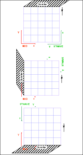 Figure14. Example CMS-M2D and STWAVE grid orientations 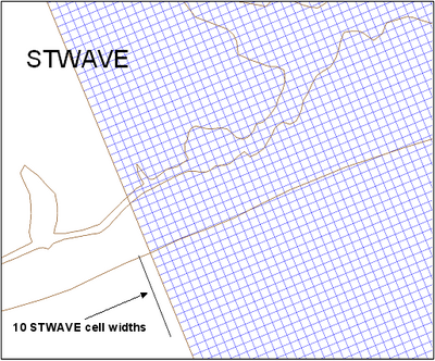 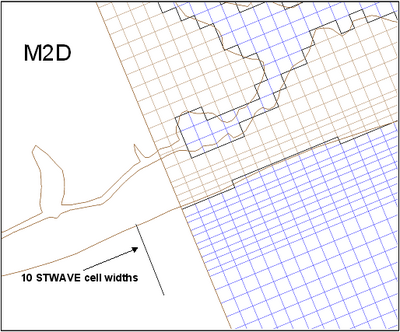 Figure15. Example CMS-M2D and STWAVE grid spacing Output OptionsCMS-M2D provides two types of output that can be selected by the user. Time series of calculated variables at specific cells, called observation cells, can be saved at user-specified time intervals. Global fields can be written at user-specified times.
All variables are output at their computational location in the cell. Thus, water-surface elevation and depth are at the cell center, the u-component of velocity, x-component of flow rate, and x-component of transport rate are at the left cell face center, and the v-component of velocity, y-component of flow rate, and y-component of transport rate are at the bottom cell face center.
Observation cell time seriesTime series of water-surface elevation, u-component of velocity, v-component of velocity, x-component of flow rate, and y-component of flow rate can be saved at observation cells. The user can specify any number of cells as observation cells. Any combination of variable output may be selected ranging from one to all five previously listed. A time interval for output must be specified, and the most accurate timing of output is achieved if the output interval is specified as an integer multiple of the calculation time step. Observation cell output will take place from the start to the end of the simulation. The SMS interface provides tools for specifying all aspects of the observation cell output. Time series of each variable selected for output is written to a separate file and values for all observation cells are included in that file. Chapter 9 describes the format and provides an example of the time series observation cell output files.
Global field outputGlobal output of scalar (water-surface elevation and depth) and vector components (velocity and sediment transport rates) can be written at user-specified times. Each variable type is written to a separate file. CMS-M2D reads two files containing times at which global output is specified, one file for scalar variables and one file for vector variables. Thus, global output times for the two variable types are not required to be concurrent, and the increment between successive times does not have to be constant. By specifying discreet time stamps, the user has flexibility for creating global files with more dense temporal resolution during certain time intervals. The SMS interface provides tools for specifying all aspects of the global output. Chapter 9 describes the format and provides an example of the global output files.
Surfacewater Modeling System Interface for CMS‑M2DCMS-M2D is supported by an interface with SMS Versions 8.0 and higher. The interface contains tools for grid development, parameter specification, control file setup, boundary specification including extraction of water-surface elevation and/or velocities from regional models such as ADCIRC, model runs, post-processing of global field values, visualization, and coupling of CMS-M2D with STWAVE or WABED through the Steering Module. This chapter provides instruction on creating and working with CMS-M2D projects within the SMS. Dialogs shown are from SMS 9.0 and 9.2.
Access to the CMS-M2D interface is obtained through the Cartesian Grid Module in the SMS. The Map Module can also be used to create simulations for CMS-M2D via a CMS-M2D Coverage. The interface for CMS-M2D includes:
Required InformationA CMS-M2D grid is a Cartesian Grid with cells that may be of varying sizes. Each cell has a location, side dimensions (Δxand Δy), and depth. Grid definition within SMS includes:
The SMS interface provides tools and methodology for the user to define each of these components and to develop the grid. Depths over the model domain are the most complex component of the grid because these values can represent any geometric shape. Bathymetric information is supplied to the SMS by the user as either a constant depth or as a spatially distributed set of data points (also known as a triangulated irregular network or TIN). Each point in the TIN has a depth associated with it. The SMS can read Digital Elevation Model (DEM) grids or scattered data point surveys and display them as a surface to show the area over which a grid will be generated. A typical scatter data set is illustrated by the red crosses in Figure 16. The SMS interpolates scattered data to the grid to define the depths at each cell. For more information on scatter data sets and the Scatter Data Module, refer to the SMS Help file or SHOALS toolbox documentation (Wozencraft et al. 2002). After defining a surface to represent the depth values, the user specifies the position, orientation, and extent of the grid using a rectangular object called a grid frame. Simple grids with constant-sized cells can be created in the Cartesian Grid Module. More complex grids are created in the Map Module. 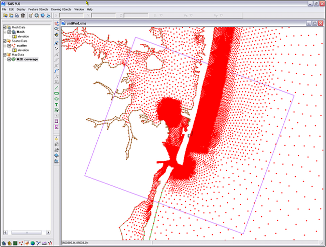 Figure 16. Grid frame around scattered data points Grid Generation from CMS-M2D CoverageMost grids will be developed within the Map Module. Information in the Map Module is stored in layers or coverages. Each coverage has a specific type, which defines the properties of the information stored in that layer. The SMS includes a CMS-M2D coverage type to allow the definition of a CMS-M2D simulation. A default coverage is in the SMS at all times. This default coverage can be used to create a CMS-M2D coverage by changing its type. Otherwise, a new coverage with type CMS-M2D can be created by left-clicking on Map Data in the Project Explorer (the data tree on the left side of screen) and then selecting New Coverage. To convert a coverage to a CMS-M2D coverage, left-click on the coverage to select it, then right-click and choose Type to expand the Coverage Type options, then select CMS-M2D. By changing a coverage to be a CMS-M2D coverage, the modeler has instructed the SMS to create a CMS-M2D grid from the information being entered.
Grid frame creation and editingWith a CMS-M2D coverage active, the grid frame is defined by selecting the Create Grid Frame tool To edit a grid frame, the modeler selects the Select Grid Frame tool
Grid frame parameters can also be explicitly modified using the edit window that appears when the grid frame is selected. These parameters are:
The grid frame size is displayed at the lower edge of the screen as it is being edited. Grid generationAfter the grid frame is defined, a CMS-M2D grid is generated in SMS with the Feature Objects | Map -> 2D Grid command. This command opens the Map->2D Grid dialog (Figure 17). For a simple grid frame, this dialog allows the user to specify the number of cells in each direction (or the cell size in each direction) and the source for depth information. The resulting grid will consist of constant-sized cells. 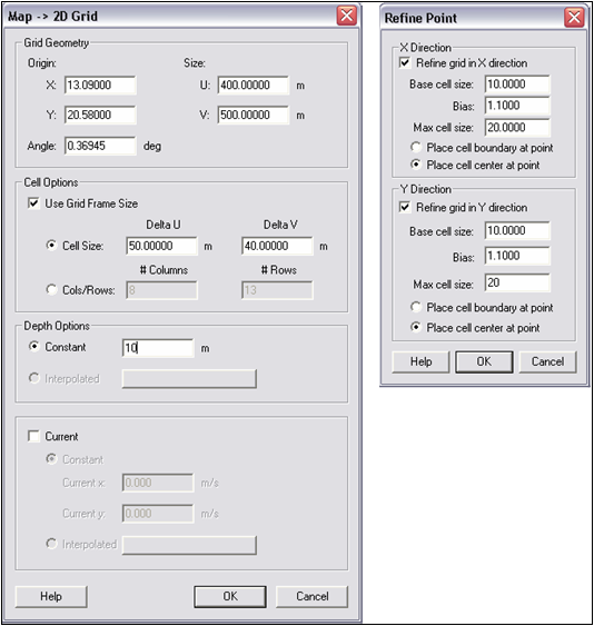 Figure17. Map-> 2D Grid and Refine Point dialogs CMS-M2D allows varying cell sizes to provide greater resolution in areas where needed. The interface provides for the development of grids with greater resolution in specific areas through the creation of refine points. A refine point is produced by creating a feature point
When refine points are present in the CMS-M2D coverage, the top portion of the Map->2D Grid dialog is dimmed out. The SMS will generate cells that match the refine point specifications. If multiple refine points are present and conflict with each other, cells will be created to meet the criteria of all refine points as closely as possible. Figure 18 shows a grid developed with a refine point in the inlet and cell strings around the grid boundary. 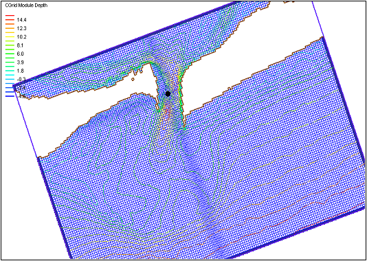 Figure18. SMS-generated CMS-M2D grid Each cell will be assigned a depth based on the depth option, and cells will be assigned to be land or water based on the resulting depths. However, the modeler may force islands, or other coastline features, into a grid by creating arcs with the Create Feature Arc tool
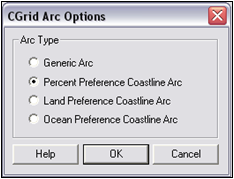 Figure19. Arc options for developing coastlines After an arc type is specified, selecting the arc will reveal the water and land sides of the arc, which are displayed as blue and brown arrows, respectively. If the water and land sides of the arc are opposite from what they should be, the arc direction can be reversed by clicking Reverse Arc Direction under the Feature Objects pull-down menu. The Map->2D Grid command also creates cell strings across all ocean boundaries of the grid. These strings are described in the following section and are tools for assigning boundary conditions for the numerical model run. Cartesian Grid ModuleThe Cartesian Grid Module contains tools for editing 2D Cartesian grids. These grids consist of cells aligned with a rectilinear coordinate system. An existing grid can be read in from a CMS-M2D simulation file, or created through the Map Module. To enter the Cartesian Grid Module from another module, select Cartesian Grid Data from the Data Tree. With a grid in memory, the following tools are available to edit the grid:
| ||||||||||||||||||||||||||||||||||||||||||||||||||||||||||||||||||||||||||||||||||||||||||||||||||||||||||||||||||||||||||||||||||||||||||||||||||||||||||||||||||||||||||||||||||||||||||||||||||||||||||||||||||||||||||||||||||||||||||||||||||||||||||||||||||||||||||||||||||||||||||||||||||||||||||||||||||||||||||||||||||||||||||||||||||||||||||||||||||||||||||||||||||||||||||||||||||||||||||||||||||||||||
| a. | Flow Rate-forcing: This type of boundary condition allows the modeler to define a time series of flow rates to be prescribed at the boundary. The time series associated with this boundary contains a list of times and flow rates in m3/s to be applied at boundary cells. Each cell contained in the cell string will have the prescribed flow rate. Time series can be developed within the SMS by entering the Define Curve dialog. Alternately, a pre-existing file can be assigned by clicking on the Browse file tab. If the Interpolate between times box is checked, CMS-M2D linearly interpolates between flow rate values at every time step. If the Interpolate between times box is not checked, boundary flow rate values are updated only at the times that they are provided in the input file. It is strongly recommended that the Interpolate between times box be checked for all simulations. |
| b. | Water-Surface Elevation (WSE) forcing: This type of boundary condition allows the modeler to define a time series of water level. The time series associated with this boundary contains a list of times and water levels (in meters) to be prescribed along the boundary. The Interpolate between times checkbox instructs CMS-M2D on how the time series water-level information is to be treated within CMS-M2D when forcing a boundary. If the Interpolate between times box is checked, CMS-M2D linearly interpolates between water-level values at every time step. If the Interpolate between times box is not checked, water-level values applied as boundary conditions are updated only at the times that they are provided in the input file. It is strongly recommended that the Interpolate between times box be checked for all simulations. |
| Two options for assigning a water-surface elevation boundary condition are available as follows: | |
| (1) | Single time series across a boundary: Time series of water-surface elevation can be developed with SMS by clicking on the Define Curve button. Alternately, a pre-existing file can be assigned by clicking on the Browse file tab. |
| (2) | Multiple time series across a boundary: Time series of water-surface elevation in which each cell in the cell string is assigned a unique value of water level can be developed in the SMS by selecting Extract from data set. If a regional model such as ADCIRC and its global water-surface elevation solution are loaded, the extract From Regional Model capability is made available as a possible source of the boundary condition. The Using Tidal Constituents option is also available which creates time series of water-surface elevations from a selection of tidal-constituent databases. If the boundary condition is to be extracted through the From Regional Model option, the SMS prompts the user to specify the source of the extracted information (a functional data set from the regional model) using the Extracted Boundary Condition dialog (Figure 21). Extraction of water-surface elevations is available for specification of boundary conditions from any regional 2D model that can be brought into SMS. |
| If the boundary condition is to be developed with the Using Tidal Constituents option, the SMS opens a dialog for specification of timing control for the extraction and a Tidal Constituents button which opens a second dialog in which specific tidal constituents can be selected from either the LeProvost (Le Provost et al. 1994) or the CMS-ADCIRC (Mukai et al. 2002) database. The starting time and date of the simulation must be entered so that the time components of the tidal constituents will correspond to the simulation. After all settings for the tidal constituents are selected, clicking OK will start the process of extracting the tidal constituents from the selected database and developing the time series boundary condition file for CMS-M2D. This option requires the grid to be defined relative to a global coordinate system. | |
| c. | Tidal-Constituent forcing: These boundary conditions apply up to eight tidal constituents to force water-surface elevations along the selected cell string. Tidal constituents are specified within the Tidal Constituent dialog accessed in the Model Control dialog. This option for tidal-constituent forcing provides CMS-M2D with amplitude and phase values that are spatially constant along a cell string. CMS-M2D then computes the temporal variation in the specified constituents internally. |
| d. | Extract WSE and Velocity (Vel) forcing: For this boundary condition type, the SMS detects if a regional model, such as ADCIRC, and its global water-surface elevation and velocity solution files have been loaded, and activates the extract capability as a possible source of the boundary condition input. If the boundary condition is assigned to be an extracted boundary condition, the SMS prompts the user to specify the source of the extracted information (a functional data set from the regional model) using the Extract Boundary Condition dialog. Both water-surface elevation and velocity from the regional model must be present to extract values for this boundary type. The velocity solution that is to be applied in the extraction is selected within the Regional Vector Model Solution field near the bottom of the dialog. Extraction of water-surface elevations and velocities is available for specification of boundary conditions from any larger-domain 2D model that can be brought into the SMS. |
File formats for use with CMS-M2D are described in Chapter 9 and Appendix A.
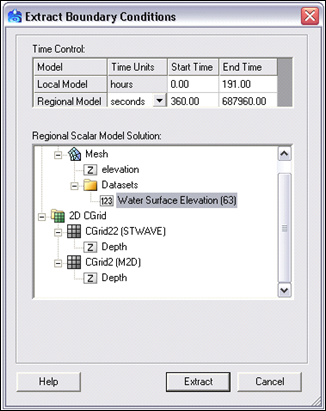
Figure21. Extract Boundary Conditions dialog
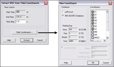
Figure22. Extract Tidal Constituents dialogs
Delete BC
The Delete BC command allows the user to delete the boundary condition assigned to a cell string. A cell string must be selected to activate this command.
Assign Cell Attributes
The Assign Cell Attributes command (Figure 23) allows the modeler to set the status for one or more selected cells. A cell can be an Inactive Land Cell, an Active Ocean Cell, an Inactive Ocean Cell, or an Observation Cell. These cell types are defined as:
Inactive Land Cell: A cell that is considered as land within the SMS and will not be saved to the CMS-M2D computational domain. If an Inactive Land Cell is adjacent to an Active Ocean Cell, the interface between the two cells will be treated as a wall.
Active Ocean Cell: A cell that is considered as water within the SMS and will be saved to the CMS-M2D computational domain. All cells in which computations are to take place must be designated as Active Ocean Cells.
Inactive Ocean Cells: A cell that is considered as water within the SMS but will not be saved to the CMS-M2D computational domain. These cells are specified adjacent to cell strings outside of the Active Ocean Cell region to denote that the area is water. This information is used by the SMS to apply correct boundary specifications in the CMS-M2D grid.
Observation Cells: An Observation Cell is a numerical station and must be assigned as an Active Ocean Cell. If a cell is specified as an Observation Cell, the Observation Cell Output Type portion of the Assign Cell Attributes dialog becomes active and the user can specify whether Time Series (water-surface elevation and velocity) or Flow Rate values are to be output as time series. Further output specifications for Observation Cells are specified in the Model Control dialog discussed later in this chapter.
The Assign Cell Attributes dialog also provides the capability to assign cells as hard bottom within the Hard Bottom Options area. To specify a cell as a hard-bottom cell, the option "Mark selected cells as non-erodible" must be checked. Then, the hard-bottom depth (maximum erosion depth) is assigned as either the cell depth or is specified as a value that is different from and greater than the cell depth. The option to specify the hard-bottom depth as a depth other than the cell depth allows for cells to start the simulation covered with sediment.
Bottom roughness can also be assigned in the Assign Cell Attributes dialog as Manning’s n.
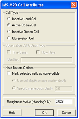
FigureMERGEFORMAT 23. Assign Cell Attributes dialog
Merge Cells
The Merge Cells command allows the modeler to merge consecutive rows or columns into one. The command is enabled only if rows or columns have been selected with the appropriate tool (select row or column).
Model Check
The Model Check command performs a number of checks on the simulation to ensure a valid model. If the system detects any missing or problematic components, it displays a message in the Model Checker dialog (Figure 24). The top portion of the dialog displays the problem while the middle and bottom sections describe the problem and a series of steps to correct the problem. When performing a model check, the SMS ensures that:
| a. | All water boundaries have boundary conditions specified. |
| b. | All observation cells have time outputs specified. |
| c. | The specified time step is less than the maximum value computed from the cell sizes and depths. |
| d. | All cell aspect ratios are less than 2. |
| e. | Correct model control specifications (i.e., if a tidal boundary exists, make sure that tidal constituents have been defined for forcing). |
| f. | No overlapping cell strings exist. |
Figure24. Model Checker dialog
CMS-M2D Model Control
The CMS-M2D Model Control command displays the Model Control dialog (Figure 25). Five tabs allow access to different model input and specification dialogs. These dialogs are:
Model Control: Set up optional input files, specify sediment transport options, and specify wave input.
Model Parameters: Specify miscellaneous parameters for wind and latitude, specify whether advection and mixing terms are invoked in momentum equation, specify whether to include wall friction, and set depth at which cells are treated as dry.
Time Control: Set up model simulation, ramp time, and hydrodynamic time step.
Output Control: Specify type and timing of hot start files, provide names for global files; provide specifications for numerical station output.
Tidal Constituents: Specify the amplitude and phase of tidal constituents if applied as boundary forcing.
A full description is provided for each dialog.
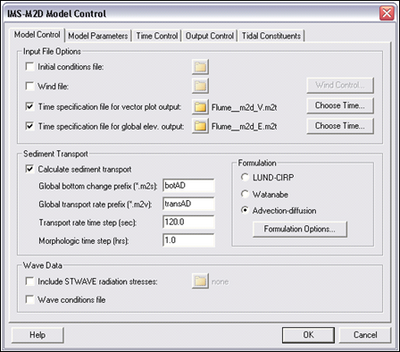
Figure25. CMS-M2D Model Control: Model Control dialog
The Model Control dialog contains three areas: Input Files Options, Sediment Transport, and Wave Data.
Input file options. Although not required, externally generated input files can be accessed in the simulation. By turning on the toggle next to each input file type, an existing file can be selected by clicking on the File Browse button. Alternatively, the user can manually create the input file by clicking on the button to the right that identifies each file type. For example, in Figure 25, an input file for time specification of vector plot output will be read by CMS-M2D, and it is called "Flume__m2d_V.m2t." Alternatively, the user can specify the time stamp information by entering the Choose Time… dialog.
Initial conditions (*.m2i). The initial conditions file contains a line for every cell in the grid containing information on the state of each cell. This information includes cell identification number, depth, water-surface elevation, u- and v-components of velocity, suspended sediment concentration,
at interior cells (boundary cells have value of 0.0),
at boundary cells (interior cells have value of 0.0), u’ and v’ (solutions of Equations 291 and 296). A full description of the initial conditions file is given in Chapter 9.
Wind (*.m2w). The wind file contains a list of time steps containing wind magnitude and direction. Each line contains three values: time (hours), magnitude (m/s), direction from which the wind is blowing (deg). Wind directions are referenced as from north = 0 deg, from east = 90 deg, etc. Note that this wind direction convention is different from the convention described for the governing equations (Chapter 2). CMS-M2D converts the wind velocity from the input file convention to the computation convention internally. Clicking the Wind Control button brings up a dialog where wind magnitude and direction time series can be specified.
Time specification for vector plot output (*_V.m2t). The Time Specification dialog allows the user to specify time stamps for global solution output (in hours). Vector plot output time specification corresponds to the global velocity and transport rate solution files (*.m2v). Time increments between global output can vary, allowing the user to have more or less frequent output.
Time specification for global elevation output (*_E.m2t). The Time Specification dialog allows the user to specify time stamps for global solution output (in hours). Scalar plot output time specification is associated with the times at which CMS-M2D will write out the global elevation and global depth files (*.m2s). Time increments between global output can vary, allowing the user to have more or less frequent output.
Sediment transport. The Calculate sediment transport option allows the user to execute sediment transport and morphology change calculations. By clicking Calculate sediment transport, file name options, sediment transport time steps, and transport formulation options become available.
Global bottom change prefix (*.m2s). The Global bottom change prefix is the prefix of the file name that will contain the global depth information (in hours), as computed by the morphology change calculations. An extension of ".m2s" is appended to the specified prefix. This global output file will be written at time stamps contained in the file specified by the Time specification for global elevation. The global depth file format contains a line with the time step, followed by subsequent lines for each grid cell with three values: x-position in present coordinate system, y-position in present coordinate system, and depth. Position values have units of meters and depth values have units of meters.
Global transport rate prefix (*.m2v). The Global transport rate prefix is the prefix of the file name that will contain the global total transport rate information (in hours). An extension of ".m2v" is appended to the specified prefix. This global output file will be written at time stamps contained in the file specified by the Time specification for vector plot. Two total load global transport rate files will be written. Instantaneous transport rates are written to a file having the Global transport rate prefix, and averaged transport rates (over time interval of dtmorph) are written to a file having "AVG" appended to the Global transport rate prefix. If the Lund-CIRP total load formulation or the AD equation is selected for sediment transport calculations, two additional global transport rate files are written, one for instantaneous bed load transport and one for instantaneous suspended load. File names for the bed load and suspended load files have "BED" and "SUS" appended to the Global transport rate prefix. Note that, if hard-bottom cells are present, the averaged total load transport rates that are saved to the file containing "AVG" have been adjusted to account for transport rate modifications owing to the presence of non-erodible substrate, but the instantaneous values contained in the remaining transport rate files contain the potential transport rate values. The global transport rate file format contains a line with the time step, followed by subsequent lines for each grid cell with four values: x-position in present coordinate system, y-position in present coordinate system, x-directed transport rate, and y-directed transport rate. Position values have units of meters, and transport rate values have units of m3/s/m.
Transport rate time step. The Transport rate time step is the time interval at which instantaneous sediment transport rates are computed in the total load formulations, and is the time interval at which the AD equation is solved and instantaneous transport rates computed if the AD formulation is applied. The transport rate time step has units of seconds.
Morphologic time step. The Morphologic time step is the time interval at which morphology change is calculated and the depth is updated. The morphologic time step has units of hours.
Formulation. If sediment transport is invoked, the user must select a transport formulation to apply. Formulation options are: Lund-CIRP total load, Watanabe total load, and AD equation and each option can be selected by clicking the radio button adjacent to it. Options specific to each formulation are accessed by clicking on the Formulation Options button. Specific parameters (Figure 26) include the median particle size, sediment density, and water density for all formulations. Each formulation also includes other parameters as shown.
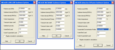
Figure26. CMS-M2D Sediment Transport Option dialogs
Wave data. Information calculated by a wave model can be entered as input to CMS-M2D in this section. The Include STWAVE radiation stresses box should be checked only if a radiation-stress gradient file is available for CMS-M2D to read in directly and the Steering Module is not invoked. This already-existing file can be selected by clicking on the File Browse button. If the Steering Module is to be run, do not check the Include STWAVE radiation stresses box as SMS will do this automatically as files become available. All other wave properties can be included in a simulation by checking the Wave Conditions box. If the Wave Conditions box is checked, CMS-M2D will read files containing wave height, period, direction, breaking index, and dissipation.
Radiation stress file (*.m2v). The radiation stress file contains the global radiation-stress gradient information (in hours). An extension of ".m2v" is customary for this file as it includes vector information, and the SMS applies this extension to radiation-stress gradient files when creating them in the Steering Module. During Steering simulations, the SMS writes radiation-stress gradient files for CMS-M2D that have values at time steps equal to the steering interval. The global radiation-stress gradient file format contains a line with the time step, followed by subsequent lines for each grid cell with four values: x-position in present coordinate system, y-position in present coordinate system, x-directed radiation-stress gradient, and y-directed radiation-stress gradient. Position values have units of meters and radiation-stress gradient values have units of m2/s2.
The Model Parameters tab of the Model Control dialog (Figure 27) contains four areas: Miscellaneous Parameters, Momentum Equation, Wall Friction, and Wetting and Drying.
Miscellaneous Parameters. This area of the dialog allows the user to specify parameters relating to wind and Coriolis calculations.
Anemometer height. If wind is specified, the height of the anemometer is required. The standard anemometer height is 10 m, and this is the default value provided by SMS. If measurements were taken with an anemometer at a different height, this height should be entered here so that CMS-M2D will convert the wind speed to wind speed at 10 m. Units for anemometer height are meters.
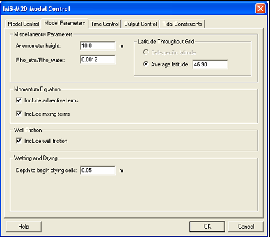
Figure27. CMS-M2D Model Control: Model Parameters dialog
Rho_atm/Rho_water. Ratio of density of air to density of water. The default value is 0.0012 and generally should not be modified.
Latitude throughout Grid. CMS-M2D applies the cell-specific latitude to compute the Coriolis term in the momentum equations. If a standard coordinate system is specified for a CMS-M2D grid, such as State Plane or UTM, the SMS will determine the latitude at the center of each CMS-M2D cell. If a local (user-defined) coordinate system is specified, the SMS does not have sufficient information to determine the cell latitudes. If cell latitudes cannot be determined by the SMS or if the user prefers to apply a single value of latitude over the grid, then a value for Average latitude can be entered that will be applied over the entire grid. Setting the latitude to zero over the entire grid will turn the Coriolis term off.
Momentum Equation. This area of the dialog allows the user to independently turn on or off the advective and mixing terms in the momentum equations. To include the advective terms, the box adjacent to Include advective terms must be checked. To include the mixing terms, the box adjacent to Include mixing terms must be checked.
Wall Friction. This area of the dialog allows the user to invoke wall friction, which is increased friction at cells having at least one wall. If the box adjacent to Include wall friction is checked, wall friction will be included in the calculations.
Wetting and Drying. This area of the dialog allows the user to specify the depth, in meters, at which CMS-M2D treats cells as dry. Typical values lie in the range of 0.03 to 0.08 m.
The Time Control tab of the Model Control dialog (Figure 28) allows specification of the start date and time, simulation duration, ramp duration, and the time step. SMS can compute a theoretical maximum time step based on celerity. Practical application of CMS-M2D requires that the time step be less than the theoretical maximum. A general guideline is to set the time step to half of the theoretical maximum, and then adjust the time step according to the hydrodynamic properties of the simulation.
Time Variables. This area of the dialog allows the user to specify time variables. The Start Date and Start Time are optional entries that do not affect the model computations or timing. The Start Date and Start Time are used only to calculate Julian Day values for time stamps for numerical station output.
Simulation Duration. The simulation duration is the total time for simulation. For example, if a simulation is to be run for 30 days, then a value of 720 hr is entered for the simulation duration. Simulation duration is given in hours.
Ramp Duration. The ramp duration is the amount of time specified for model spin-up. A typical ramp duration for an applied project is 1 day. Ramp duration is given in days.
The Output Control dialog (Figure 29) provides options for hot starts, global output files, and numerical station output files.
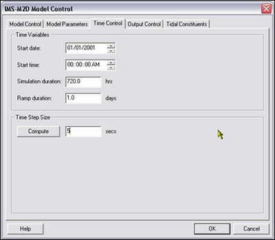
Figure28. CMS-M2D Model Control: Time Control dialog
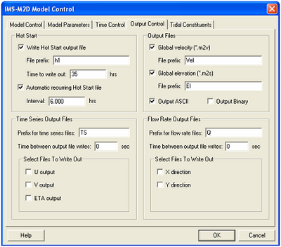
Figure29. CMS-M2D Model Control: Output Control dialog
Hot Start. Two independent hot start options are available for CMS-M2D. Checking the Write Hot Start Output File box allows the user to specify a time at which a file of the same format as the initial conditions file will be written. The hot start file can be later used as an initial conditions file for subsequent model runs. The user specifies a prefix for the hot start file name and the elapsed time, in hours, at which the file will be written. By checking the Automatic Recurring Hot Start File box and providing a time interval (hours), hot start files will be written at the time interval specified. Hot start files are written with file names alternating with HOTSTART1.M2I and HOTSTART2.M2I. These files can be later input as initial conditions files for a subsequent simulation. The file HOTSTART.INFO is also written and contains the name (HOTSTART1.M2I or HOTSTART2.M2I) and time of the last saved hot start file.
Output Files. Global velocity and elevation output file names are specified in this section of the dialog. CMS-M2D supports two types of global output, vector and scalar for each cell in the grid. Traditionally this output has been stored in ASCII files defined for the model. These ASCII files (described below), can become very large. Another option added in this version of the model is to save the same output into a binary formatted XMDF file. The user can elect to save ASCII, Binary, or both file types by checking the boxes for "Output ASCII" and/or "Output Binary." Description of the XMDF formats can be found at http://www.wes.army.mil/ITL/XMDF.
Global velocity (*.m2v). By checking this toggle box, a global velocity solution will be written out by CMS-M2D at the times specified in the CMS-M2D Output Time Specification dialog for Vector Plot. The file extension ".m2v" is appended to the prefix specified. The global velocity file format contains a line with the time step, followed by subsequent lines for each grid cell with four values: x-position in present coordinate system, y-position in present coordinate system, u-component of velocity, and v-component of velocity. Position values have units of meters and velocity values have units of meters per second.
Global elevation (*.m2s). The explanation provided for Global velocity applies here as well, with the difference being that a global elevation solution will be written out. The global elevation file format is the same as that of the global velocity solution file, with the exception that the u- and v-component velocity values are replaced by the water level in meters at each cell.
Time Series Output Files. This section allows the user to specify output options for numerical stations where water-surface elevation and/or velocity are to be saved at equal time increments. A prefix for the file containing the numerical station output must be specified. The file extension ".m2o" is appended to the specified prefix. Entering a non-zero time increment, in seconds, provides the output timing. Note that this time increment should be an integer multiple of the hydrodynamic time step. Check the variables that are to be output (u, v, or η). The ".m2o" output file will contain a header line that indicates that the first column of information is the time stamp (in Julian Day or elapsed time in days), and the list of cells at which time series values are output. The second and following lines contain the time stamp in the first column, following by values for each numerical station.
Flow Rate Output Files. This section allows the user to specify output options for numerical stations where directional components of the flow rate are to be saved at equal time increments. A prefix for the file containing the numerical station output must be specified. The file extension ".m2o" is appended to the specified prefix. Entering a non-zero time increment, in seconds, provides the output timing. Note that this time increment should be an integer multiple of the hydrodynamic time step. Check the directional flow components that are to be output (x and/or y-directed flow rate). The ".m2o" output file will contain a header line that indicates that the first column of information is the time stamp (in Julian Day or elapsed time in days), and the list of cells at which time series values are output. The second and following lines contain the time stamp in the first column, following by values for each numerical station.
The Tidal Constituents dialog (Figure 30) allows the user to select up to eight tidal constituents to apply as forcing in CMS-M2D. The user must specify the local amplitude and phase of each tidal constituent. Amplitude and phase is held spatially constant along an entire cell string for each tidal constituent. Phase must be specified in the same time zone as other model inputs. Amplitude and phase values for the eight constituents can often be obtained from National Ocean Service harmonic analysis for local water-level gauges.
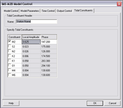
Figure30. CMS-M2D Model Control: Tidal Constituents dialog
Run CMS-M2D
The Run CMS-M2D command makes sure the current simulation is saved to disk, and launches CMS-M2D to run the present simulation. The SMS also performs a model check before launching the model. If any anomalies are detected, a warning is issued.
Steering Module
Coupling of CMS-M2D with STWAVE (or WABED) is conducted through the Steering Module. This feature controls interaction of the two models by alternating STWAVE and CMS-M2D runs for a specified time called the Steering Interval, and provides mapped fields of variables to each model. The user controls the steering options by checking boxes in the Steering Module dialog for each type of interaction needed for the specific simulation (Figure 31).
To invoke the Steering Module, CMS-M2D and STWAVE (or WABED) grids must be loaded into SMS. All inputs and options for both models must be specified before launching the steering process. Users should consult the STWAVE User’s Manual (Smith et al. 1999, 2001) for information on setting up STWAVE in SMS. WABED can be set up with the same tools and conventions as STWAVE.
The Steering Module dialog is opened from the Data drop-down menu (Figure 31). The steering interval is set by specifying the time requested by the "Run" inquiry. Interaction between the models is selected by clicking the available options in the CMS-M2Dà STWAVE/WABED (meaning CMS-M2D passes velocities and/or total depth to STWAVE or WABED) and STWAVE/WABEDàCMS-M2D (meaning STWAVE or WABED passes wave information to CMS-M2D) portions of the dialog. If sediment transport calculations are invoked, the Steering Module will always pass updated depths from CMS-M2D to STWAVE or WABED so that modifications of the waves owing to morphology change will be taken into account. If the "Wave Conditions" box is checked in the CMS-M2D Model Control dialog (Figure 25), the Steering Module will map fields of wave properties (height, period, wave direction, breaking index, and wave dissipation) to the CMS-M2D grid for inclusion in hydrodynamic and sediment transport calculations.
After the Steering Module setup is complete, clicking Start invokes the steering process. If the SMS detects that a previous steering run has been conducted for the present project, a Restart Options (Figure 32) dialog will pop up to allow the user to specify whether to continue the previous steering simulation or start at the beginning of the steering process. If the user chooses to restart from a previous steering simulation, the dialog allows options to select which model simulation and steering interval to start from. Once the steering process has been initiated, a progress screen will be shown.
During steering, the SMS creates two output files that provide information on the steering process and on the model progress. The file "steeringstatus.txt" provides information on the steering options and status of the steering process. The file "screenoutput.txt" contains text that CMS-M2D and STWAVE or WABED write to the screen. If the steering simulation is unsuccessful, the user is advised to examine these two files to help determine the source of the problem.
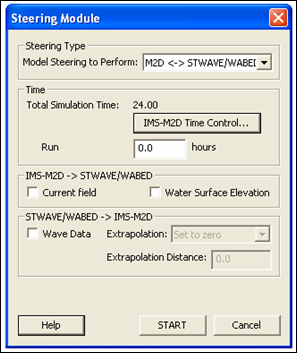
Figure31. Steering Module dialog
Figure32. Steering Module Restart Options dialog
Saving a Project
During development of a project within the SMS, numerous sets of information may be brought in and applied to grid development and simulation setup. It is common for a CMS-M2D project to contain bathymetric data, Map Module information such as a grid frames and refine points, a CMS-M2D grid and model setup, an STWAVE or WABED grid and model setup, and an ADCIRC (or other regional model) mesh and solution files from which CMS-M2D boundary conditions have been extracted. In addition, the coordinate system in which the grids have been developed is contained with the SMS information. The SMS will save all of the information collectively as a project by using the Save Project option or Save As and then choosing the ".sms" option. When saved as a project, SMS will create a master project file with the ".sms" extension that saves all information related to the project. When a project file is loaded into SMS, all scatter data, map information, and models that were previously contained in the project will be loaded.
The user may opt to save information specific to a particular module or model. For example, to save a CMS-M2D model setup, the SMS will issue a Save M2D command from the File drop-down menu if a CMS-M2D simulation is selected in the Data Tree.
Model Setup and File Structure
Setup of CMS-M2D requires development of a computational grid and preparation of one or more input files. The SMS creates all model input files in the correct format so that editing or input file generation is generally not required. The exceptions to this are preparation of time series of wind speed and direction, water level, or flow rate files for input as forcing. These files can be created within the SMS, but often the user already possesses data from which these files are developed. This section describes the structure of files required to run the CMS-M2D model and its output files to assist the user in understanding the file formats. All input and output files to CMS-M2D are ASCII. Unless otherwise noted, files are free format. ===Input Files===
Required input files for CMS-M2D are the grid file, control file, and one or more forcing files (boundary conditions, wind input, or radiation-stress gradient input). A particular simulation may require additional input files that can include any combination of initial conditions, water-level time series, flow rate time series, tidal constituents, wind speed and direction, waves stress, wave properties, sediment transport options and parameters, specifications for non-erodible cells, and output specification. Structures of these input files are described here. Sample files are provided in Appendix A.
Grid file
The grid file for CMS-M2D is structured such that all information pertaining to a cell is found on the same line as the cell identification number. This format is convenient for the user so that once a cell is located in the grid file, its properties are easily viewed. The grid file contains some information that is not used within CMS-M2D, but is retained for user reference and post-processing.
The first line of the grid file is a header line that describes the columns of information that make up the grid. All lines after the first specify cell information. Cells are defined by their cell identification number and the cell numbers of adjacent cells, referred to by local direction (north, east, south, west). These directions are relative to the local (grid) coordinate system defined by the grid, which may or may not be aligned with global geographic coordinates. With respect to the local grid system, north refers to the positive y direction and east refers to the positive x direction.
Each line describing a cell consists of the following information: Cell number, NC, EC, SC, WC, NB, EB, SB, WB, IACTV, DX, DY, H, N, ROW, COL, LAT, X-DIST, Y-DIST
Descriptions of parameters are given in Table 4 and details of the cell activity parameter (IACTV) are given in Table 5.
| Definitions of Parameters in Grid File | |||
| Parameter | Description1 | ||
| Cell Number | Cell identification number (referred to as ICELL within CMS-M2D) | ||
| NC | Cell number of cell adjacent to and north of ICELL | ||
| EC | Cell number of cell adjacent to and east of ICELL | ||
| SC | Cell number of cell adjacent to and south of ICELL | ||
| WC | Cell number of cell adjacent to and west of ICELL | ||
| NB | Boundary type at northern edge of ICELL | ||
| EB | Boundary type at eastern edge of ICELL | ||
| SB | Boundary type at southern edge of ICELL | ||
| WB | Boundary type at western edge of ICELL | ||
| IACTV | Cell type or active status | ||
| DX | Cell width parallel to the x-axis (m) | ||
| DY | Cell width parallel to the y-axis (m) | ||
| H | Still-water depth relative to a user-specified datum (m) | ||
| N | Manning roughness coefficient (m/s1/3) | ||
| ROW | Row position of cell2 | ||
| COL | Column position of cell2 | ||
| LAT | Latitude (decimal degrees) | ||
| X-DIST | X coordinate or distance from grid origin (m) 3, 4 | ||
| Y-DIST | Y coordinate or distance from grid origin (m) 3, 4 | ||
| 1. Directional description (north, east, south, west) refers to the grid coordinate system. 2. Parameter is not applied in CMS-M2D calculations. 3. Parameter is not applied in CMS-M2D calculations, but is written in global output files. 4. Coordinates are located at cell centers. | |||
| Cell Types and Their Function in CMS-M2D | ||
| Type Index (IACTV) |
Type | Function |
| 0 | Inactive | Cell not included as part of calculation domain. |
| 1 | Active regular cell | Non-forcing, regular cell. |
| 2, 6 | Water-level forcing boundary cell | Water level specified as a boundary condition at this cell. Type indices of 2 and 6 denote whether the forcing file contains an individual time series (Type Index = 2) or multiple time series (Type Index = 6). |
| 3 | Flow-rate forcing boundary cell | Flow rate specified as a boundary condition at this cell. |
| 5 | Tidal-constituent forcing boundary cell | Water-level specified through tidal constituents as a boundary condition at this cell. |
| 7 | Mixed water-level and velocity forcing cell | Water level and velocity applied as boundary condition at this cell. Requires multiple time series file. |
Cell-center coordinates (x-dist and y-dist) can be given in any Cartesian coordinate system, such as State Plane or UTM. CMS-M2D does not apply the cell-center coordinates in calculations, but does export the values in global files of water-surface elevation and velocity. Because no specific coordinate system is required, the user can apply a coordinate system that is convenient for the particular application.
A grid file is required for all CMS-M2D projects. SMS saves CMS-M2D grid files with the extension ".m2g."
Model control
Model control specifications are defined in an input file called "m2d.m2c" or "projectname.m2c" where "projectname" is given to SMS by the user. SMS saves the control file as "m2d.m2c" and as "projectname.m2c." Each line of the control file contains the parameter or character string followed by a description. The description is informational and CMS-M2D does not read it. File names for input and output are user specified for CMS-M2D, with the exception of the alternating hot-start files, and are listed as input parameters in the control file. Names of files are limited to 50 characters and cannot contain spaces. There must be at least one space between the parameter or character string and the description. Information contained in the control file is listed in Table 6 in the required order. The format of the control file is the same for all model and project configurations. All parameters listed in Table 6 must be included in the control file.
Two types of output files can be specified: time-series of variables at specified cells, and global values of variables at specified times. To specify time-series of variables, cell numbers are identified at locations to output information and a separate file is created to save each variable. Files denoted in Table 6 as "Cell-specification files" list cell identification numbers at which time series information is stored. Each line of a cell-specification file contains one cell identification number.
Files denoted in Table 6 as "Time-specification files" are for global velocity and elevation output, and contain a list of times to save data. Times are specified as elapsed hours since the beginning of the simulation. Each line in the file contains one value of time and times must be in sequential order. The interval between successive outputs can vary through the simulation. For example, a time specification file may have output times prescribed as 0, 1, 2, 2.5, 3, 3.5, 4, 4.25, and 5 hr.
| Model Control File Specifications | ||
| Parameter | Description | |
| Version | CMS-M2D Version number | |
| Anemometer height (m) | Height of anemometer above water or land surface | |
| Output file format | Specification of CMS-M2D output file type. Options: BINARY, ASCII, or BOTH | |
| Angle between true north and y-axis of grid (deg) | Defined by grid orientation | |
| Grid origin x-coordinate | Location of x position of cell 1 | |
| Grid origin y-coordinate | Location of y position of cell 1 | |
| Time step (s) | Model time step | |
| Automated hot-start interval (hr) | Time interval between automated hot-start file writes | |
| Include advective terms | Flag for inclusion of advective terms in the momentum equation. Flag settings: 0 = do not include, 1 = include | |
| Include mixing terms | Flag for inclusion of mixing terms in the momentum equation. Flag settings: 0 = do not include, 1 = include | |
| Include wall friction | Flag for calculation of wall friction at cells with wall faces. Flag settings: 0 = do not calculate wall friction, 1 = calculate wall friction. | |
| Depth (m) to begin drying cells | Drying will occur if the total depth in a cell is less than or equal to the depth specified here. | |
| Calculate sediment transport | Flag for calculation of sediment transport. Flag settings: 0 = do not calculate, 1 = calculate | |
| Starting Julian Day (YYDDD OR DDD) | Date of beginning of simulation | |
| Start time (hr) | Time of beginning of simulation | |
| Realization time (hr) | Duration of simulation | |
| Ramp duration (day) | Duration of ramp | |
| (Sheet 1 of 3) | ||
---- Table 6 (Continued) | ||
| Parameter | Description | |
| Steering Module elapsed time | Cumulative time at beginning of present simulation; applied for multiple simulations with Steering Module | |
| Time to write output for hot-start (hr) | Time when hot start output is to be written. Use a value of 0 if no hot-start information is to be saved. | |
| Grid file name | Name of grid file (required) | |
| Initial conditions file name | Name of file containing initial conditions. If starting the simulation from quiescent conditions, use "default" (without the quotes) instead of a file name. | |
| Tidal constituents file name | Name of file containing tidal constituents. | |
| Wind input file name | Name of file containing wind speed and direction (required). | |
| Include radiation stresses | Flag for inclusion of radiation stress forcing. Flag settings: 0 = no radiation stress forcing, 1 = include radiation stress forcing. | |
| Wave properties file | Name of a file containing the names of wave-properties files for height, period, direction, breaking, and dissipation1. | |
| Radiation stress file | Name of radiation stress file1.rad. | |
| Hot-start output file name | Name of hot start output file1. | |
| Time-specification file for vector plot output | Name of file containing times for vector plot (global u, v) output1. | |
| Time-specification file for global elevation output | Name of file containing times for global elevation output1. | |
| Time-series output cell-specification file | Name of file containing cell numbers for time-series output of u, v, h1. | |
| Flow rate output time-series cell-specification file | Name of file containing cell numbers for flow rate output1. | |
| Time between output file writes (s) for u, v, h time-series file | Time should be a multiple of the simulation time step. | |
| Time between output file writes (s) for flow-rate file | Time should be a multiple of the simulation time step. | |
| Time-series output file for u | Name of file to contain u time series1. | |
| Time-series output file for v | Name of file to contain v time series1. | |
| Name of file to contain h time series1. | ||
| Flow rate output file for Qx | Name of file to contain time series of Qx1. | |
| Flow rate output file for Qy | Name of file to contain time series of Qy1. | |
| Prefix for vector output file name | CMS-M2D appends ".m2v" to the user-specified prefix when naming the vector output file. | |
| Prefix for global elevation output file name | CMS-M2D appends ".m2s" to the user-specified prefix when naming the global elevation file. | |
| (Sheet 2 of 3) | ||
| Table 6 (Concluded) | |
| Parameter | Description |
| Prefix for global depth output file name | CMS-M2D appends ".m2s" to the user-specified prefix when naming the global depth file. |
| Prefix for transport rate output file name | CMS-M2D appends ".m2v" to the user-specified prefix when naming the global transport rate file. |
| HDRIVER file name | Name of file containing water-surface elevation forcing information (individual time-series files). |
| QDRIVER file name | Name of file containing flow rate forcing information. |
| MHDRIVER file name | Name of file containing water-surface elevation forcing information (multiple time-series files). |
| MVDRIVER file name | Name of file containing velocity forcing information (multiple time-series files). |
| (Sheet 3 of 3) | |
| 1. Use "none" or "NONE" if no hot-start output for this variable is specified. | |
Initial conditions
An initial-conditions file provides information at the beginning of the simulation at all cells. Each line in the initial-conditions file contains 15 values. The first ten are cell number, ambient depth, water-surface elevation, u- and v-components of velocity, suspended sediment concentration, ![]() at interior cells (boundary cells have value of 0.0),
at interior cells (boundary cells have value of 0.0),![]() at boundary cells (interior cells have value of 0.0), u’, and v’. Depth and water level are given in m, velocity components are given in m/s,
at boundary cells (interior cells have value of 0.0), u’, and v’. Depth and water level are given in m, velocity components are given in m/s,![]() values are given in m/s, and concentration is given in m3/m3. The 11th through 14th values are the cell boundary type indices (Table 4), and the 15th column is the cell activity parameter (IACTV). CMS-M2D writes hot-start files in the correct format for reading as initial conditions. If a time-specific hot start is specified within the SMS model control, the hot-start file name will have the extension ".m2i." If the automatic recurring hot-start capability within CMS-M2D is invoked, the hot-start files will be named "HOTSTART1.M2I" and "HOTSTART2.M2I." Automatic hot-starts are invoked by setting the hot-start time interval to a value, in hours, greater than zero.
values are given in m/s, and concentration is given in m3/m3. The 11th through 14th values are the cell boundary type indices (Table 4), and the 15th column is the cell activity parameter (IACTV). CMS-M2D writes hot-start files in the correct format for reading as initial conditions. If a time-specific hot start is specified within the SMS model control, the hot-start file name will have the extension ".m2i." If the automatic recurring hot-start capability within CMS-M2D is invoked, the hot-start files will be named "HOTSTART1.M2I" and "HOTSTART2.M2I." Automatic hot-starts are invoked by setting the hot-start time interval to a value, in hours, greater than zero.
Water-level forcing data files
Time-series boundary forcing for CMS-M2D can be specified as water-surface elevation. Two types of files containing water-surface elevation forcing information can be applied. One type contains individual time series and the other type contains multiple time series. Both individual and multiple time series forcing can be applied in the same simulation. This capability is convenient for situations in which the time increment is not equal between different sets of time series. This capability also provides flexibility for defining multiple water-level forcing cell strings within the SMS and specifying forcing from various sources. For example, a simulation may require that one or more cell strings are forced by data from a water-level gauge and use the individual forcing file, and also that one or more cell strings are forced by water levels calculated by a regional model or tidal-constituent database and saved in a multiple time-series file.
CMS-M2D recognizes whether time series of water level are specified as forcing by identification of forcing cells in the grid file. If time series water-level driving cells are found, CMS-M2D opens the HDRIVER and/or MHDRIVER files (see Table 6). The first line of the HDRIVER or MHDRIVER file contains two integer values. The first value specifies the number of files containing water-surface elevation forcing time series. The second value is the total number of cells forced by water-surface elevation values for HDRIVER files, and is the maximum number of cells forced by water-surface elevation for MHDRIVER.DAT files. More than one multiple time series file can be applied in a simulation. The maximum number of cells forced by water-surface elevation is the greatest number of cells forced for all files listed in the MHDRIVER.DAT file.
The second line contains the name of a data file that contains the forcing data. The third line of the HDRIVER or MHDRIVER.DAT file contains the number of cells that are driven by the data contained in the file listed in the second line, and an interpolation parameter. The interpolation parameter specifies whether or not the forcing data are interpolated between model time steps. For example, water-level forcing data may be available every hour, but the model time step might be 30 s. If the interpolation parameter is set to 1, values of water level at the forcing boundaries are interpolated at each model time step. If the interpolation parameter is set to 0, no interpolation takes place. Following the first and second lines a list of cell numbers that are forced by the time series data given in the forcing data file. For the individual time series forcing files, all cells in the list are forced by the same single time series. Cells forced by water levels contained in the multiple time series file must be listed in the MHDRIVER.DAT file in the order that their corresponding time series appear in the forcing data file.
If more than one forcing data file is applied for water level or discharge, information is specified exactly as previously described for all sets of forcing data and placed in the HDRIVER or MHDRIVER file below the information for the first file.
If boundary input is specified as individual time series of water-surface elevation in a CMS-M2D project, the SMS saves the HDRIVER file name as "hdriver_projectname.dat." If boundary input is specified as multiple time-series of water-surface elevation in a CMS-M2D project, the SMS saves the MHDRIVER file name as "mhdriver_projectname.dat."
Files containing individual time series water-level forcing data (listed in HDRIVER.DAT) are specified to have two values on each line. The first value is the time stamp. The time is specified in hours since the beginning of the simulation. So, at t = 0, the time stamp would be 0.0 and at t = 1 day, the time stamp would be 24.0. The second value is water-surface elevation (m) relative to the same datum as the grid for water-level forcing data, or flow rate (m3/s) for discharge data. Time stamps must start at 0.0 and end at or after the ending time of the simulation.
Files containing multiple time-series water-level forcing data (listed in MHDRIVER.DAT) must have on each line a time stamp followed by a water-level value for each of the cells listed that correspond to the particular forcing file. Thus, if J cells are to be forced with a particular multiple time series file, then J+1 columns must be present in the forcing file. Columns of water-level values must be listed in the same order as the cell numbers are listed in the MHDRIVER.DAT file. The time is specified in hours since the beginning of the simulation. So, at t = 0, the time stamp would be 0.0 and at t = 1 day, the time stamp would be 24.0. Water-surface elevation (m) is provided relative to the same datum as the grid for water-level forcing data. Time stamps must start at 0.0 and end at or after the ending time of the simulation.
The SMS contains dialogs in which time series of water-surface elevation and flow rate can be prescribed for CMS-M2D. If these dialogs are accessed to create the time series files, they will be saved with the extension ".wl."
Velocity forcing data files
Forcing by velocity information can be applied in conjunction with the multiple time series water-level forcing. The velocity format is also a multiple time series. Velocity time series cannot be specified without water-level forcing at the same cells.
CMS-M2D recognizes whether time series of combined water-level and velocity values are applied as forcing by identification of forcing cells in the grid file. If time series combined water-level and velocity driving cells are found, CMS-M2D opens the MHDRIVER and MVDRIVER files (see Table 6). The file format for the MVDRIVER file is identical to that of the MHDRIVER file described in the previous section of this chapter. SMS saves the MVDRIVER file as "mvdriver_projectname.dat."
Files containing multiple time series velocity forcing data (listed in MVDRIVER.DAT) must have on each line a time stamp followed by four velocity values for each of the cells listed that correspond to the particular forcing file. Velocities written for each cell are those on the cell faces and are written in the following order: uleft, uright, vbottom, vtop where the subscripts left, right, bottom, and top denote the cell faces in the grid coordinate system. Thus, if J cells are to be forced with a particular multiple time series file, then 4*J+1 columns must be present in the forcing file. Columns of sets of velocity values must be listed in the same order as the cell numbers are listed in the MVDRIVER.DAT file. The time is specified in hours since the beginning of the simulation. So, at t = 0, the time stamp would be 0.0 and at t = 1 day, the time stamp would be 24.0. Time stamps must start at 0.0 and end at or after the ending time of the simulation.
The SMS contains a dialog in which time series of combined water-surface elevation and velocity can be prescribed for CMS-M2D in which the boundary values are obtained from the solution of a larger-domain model. The SMS automatically maps the solution to the CMS-M2D cells.
Flow rate forcing data files
Flow rate is forced by files containing individual time series information. CMS-M2D recognizes whether time series flow rate values are applied as forcing by identification of forcing cells in the grid file. If time series flow rate driving cells are found, CMS-M2D opens the QDRIVER file (see Table 6). The first line of the QDRIVER file contains two integer values. The first value specifies the number of files containing flow rate forcing time series. The second number is the total number of cells forced by flow rate.
The second line contains the name of a data file that contains the forcing data. The third line of the QDRIVER file contains the number of cells that are driven by the data contained in the file listed in the second line, and an interpolation parameter. The interpolation parameter specifies whether or not the forcing data are interpolated between model time steps. For example, flow rate forcing data may be available every hour, but the model time step might be 30 s. If the interpolation parameter is set to 1, values of flow rate at the forcing boundaries are interpolated at each model time step. If the interpolation parameter is set to 0, no interpolation takes place. Following the first and second lines of the QDRIVER file is a list of cell numbers that are forced by the time series data given in the forcing data file.
If more than one forcing data file is applied for flow rate, information is specified exactly as previously described for all sets of forcing data and placed in the QDRIVER file below the information for the first file.
If time series of water-surface elevation is specified in a CMS-M2D project, the SMS saves the QDRIVER file name as "qdriver_projectname.dat."
Files containing flow rate forcing data are specified to have two values on each line. The first value is the time stamp. The time is specified in hours since the beginning of the simulation. So, at t = 0, the time stamp would be 0.0 and at t = 1 day, the time stamp would be 24.0. Time stamps must start at 0.0 and end at or after the ending time of the simulation. The second value is flow rate given in m3/s. This flow rate is specified at every cell designated as forced by the input series in the QDRIVER file. Thus, if three cells were specified as flow rate forcing cells and the value of the flow rate was 9 m3/s, then each of the three cells would have 9 m3/s flowing through it. The flow rate is not distributed among the three cells.
The SMS contains a dialog in which time series of flow rate can be prescribed for CMS-M2D. If this dialog is accessed to create the time series files, they will be saved with the extension ".q."
Wind speed and direction
Wind speed and direction are given in the user-specified wind file listed in the model control file (*.m2c). The wind-forcing file contains three values on each line. The first value is the time stamp in hours since the beginning of the simulation. The second value is the wind speed in m/s and the third value is direction in deg. The convention for the input wind direction is 0 deg indicates wind blowing from the north, and 90 deg indicates wind blowing from the east. Wind speed must be positive. Conversion to the wind-direction convention given for Equations 2 and 3 is conducted internally within CMS-M2D.
The SMS contains a dialog in which time series of wind speed and direction can be prescribed for CMS-M2D. If this dialog is accessed to create the time series file, it will be saved with the extension ".m2w."
Tidal constituents
The tidal-constituent forcing file contains nine lines. The first line is a header that can identify the source of the tidal-constituent information. The header line is ignored by CMS-M2D. Each of the remaining lines contain the local amplitude (m) and phase (deg) of the water level for a specific tidal constituent. The constituents specified on lines 2 through 9 are (in order of appearance): M2, N2, S2, K2, K1, O1, M4, and M6. If specific constituents are not to be specified as forcing, then their amplitude values must be set to zero.
Wave stresses
Wave stresses are given in the user-specified radiation-stress file listed in the model control file. The radiation-stress file consists of sets of wave stresses prescribed at specific times. The first line in the file contains the text "TIME:" and is followed by the time in hours since the beginning of the simulation. Lines 2 through NCELLS + 1 contain three values. The first value is the cell identification number and the second and third values are the x and y components of the wave stress, respectively. Wave stresses must be given in order of ascending cell identification numbers. Sets of information that include the time step and wave stresses for each cell are included in the file for each time step for which wave stresses are available. Because CMS-M2D will conduct its calculations at a different time interval than the wave stress time interval, the stresses are linearly interpolated within CMS-M2D over time. If the last time stamp in the wave stress file specifies a time before the end of the CMS-M2D simulation, CMS-M2D will apply values of zero for the radiation stresses after the time of the last available wave information (no interpolation to zero is conducted).
If the Steering Module is invoked to couple CMS-M2D with STWAVE (or WABED), SMS will write files containing wave stresses that have been mapped from those calculated by the wave model. SMS gives the extension ".rad" to the wave stress file. The same file extension is also given to radiation stress files for STWAVE. CMS-M2D files can be distinguished from the STWAVE files by the prefix. CMS-M2D wave stress files contain the text "m2steer" and the STWAVE files contain "swsteer."
Wave properties file
The wave properties file contains a list of five file names with each line containing one file name. The files must be listed in the order of wave height, wave period, wave direction, wave breaking index, and wave dissipation. Each of the files listed contains fields of the specified wave property. If SMS generates the wave properties file, it specifies an extension of ".mwv."
Wave height, period, direction, breaking index, and dissipation are provided as time series of fields in unique files (one wave property per file). Each file consists of sets of the wave property prescribed at specific times. The first line in the file contains the text "TIME:" and is followed by the time in hours since the beginning of the simulation. Lines 2 through NCELLS + 1 contain two values. The first value is the cell identification number, and the second value is the wave property. Values of wave properties must be given in order of ascending cell identification numbers. Sets of information that include the time step and wave properties for each cell are included in the file for each time step that wave properties are available. Because CMS-M2D will conduct its calculations at a different time interval than the wave property time interval, the property is linearly interpolated within CMS-M2D over time.
Sediment transport and morphology change specifications file
The file providing the sediment transport and morphology change specifications contains information on timing control for transport and morphology change calculations, specification of the transport formulation to apply, general parameter settings, and parameter settings specific to the selected transport formulation. Because each transport formulation requires a unique set of inputs, the format for this file varies depending on the chosen formulation. This file is required to have the name "sedparams.dat."
If the Watanabe sediment transport formulation is specified, the sedparams.dat file will contain ten lines, each having a single value. The first line will have an integer value of 1, which is an index that informs CMS-M2D to apply the Watanabe transport formula. The second and third lines contain the sediment transport rate time step (sec) and the morphology change time step (hr), respectively. The fourth, fifth, and sixth lines contain the median grain size (mm), sediment density (kg/m3), and the water density (kg/m3), respectively. The seventh line contains the transport rate slope coefficient Ds (unitless) of Equations 112 and 113. Line 8 contains the critical threshold for sediment movement transport. Lines 9 and 10 contain the transport rate coefficient A0 of Equations 112 and 113, and sediment porosity p, respectively.
If the Lund-CIRP sediment transport formulation is specified, the sedparams.dat file will contain 12 lines, each having a single value. The first line will have an integer value of 2, which is an index informing CMS-M2D that the Lund-CIRP transport formula is to be applied. The second and third lines contain the sediment transport rate time step (sec) and the morphology change time step (hr), respectively. The fourth, fifth, and sixth lines contain the median grain size (mm), sediment density (kg/m3), and water density (kg/m3), respectively. Line 7 contains the water temperature (deg C). Line 8 contains the transport rate slope coefficient Ds (unitless) of Equations 112 and 113. Line 9 contains the flag denoting whether or not ripples are included in the calculations; a value of 0 indicates that ripples are not included, and a value of 1 indicates that ripples will be included. Line 10 contains the sediment porosity. Lines 11 and 12 contain the scaling factors for the bed load and suspended load, respectively.
If the AD equation is selected as the sediment transport formulation, the sedparams.dat file will contain 13 lines, each having a single value. The first line will have an integer value of 3, which is an index informing CMS-M2D that the AD equation is to be applied to compute the sediment transport rate. The second and third lines contain the sediment transport rate time step (sec) (time step at which the AD equation is solved) and the morphology change time step (hr), respectively. Lines 4 through 7 contain the median particle diameter (mm), sediment density (kg/m3), water density (kg/m3), and water temperature (deg C), respectively. Line 8 contains the slope coefficient for Equations 115 and 116. Line 9 contains the flag denoting whether or not ripples are included in the calculations; a value of 0 indicates that ripples are not included, and a value of 1 indicates that ripples will be included. Line 10 contains the sediment porosity. Line 11 contains an index that specifies the type of suspended concentration profile in which a value of 1 denotes an exponential profile with the depth-averaged mixing coefficient of Van Rijn, a value of 2 denotes a Van Rijn profile with Van Rijn’s mixing coefficient, and 3 denotes an exponential profile from the Lund-CIRP formulation. Lines 12 and 13 contain the scaling factors for the bed load and suspended load, respectively.
Non-erodible cell specifications file
The non-erodible cell specifications file contains the number of non-erodible cells in the computational grid, followed by a listing of the hard-bottom cell identification number and depth of hard substrate. One cell identification number and its corresponding hard substrate depth are listed on each line. If hard-bottom cells do not exist on the grid, the file will contain a value of zero for the number of non-erodible cells. This file is required to have the name "noerode.dat."
Selected cell output specification file
User-specified observation cells can be selected for time series output of variables or terms in the governing equations. A listing of these cells is provided in a cell output specification file. The file contains a list of cell identification numbers with one number per line. If observation cells are selected within the SMS and saved as part of a CMS-M2D project, the SMS gives the cell listing file the extension of ".ts."
Global output time specification files
Global water-surface elevation, velocity, depth, and sediment transport rates are written to files at times specified in the global output time-specification files. These files consist of a list of times, in hours since the beginning of the simulation, at which global output is to be written. Each line in these files consists of one time value. Separate global output time-specification files are required for water-surface elevation and velocity, providing the option to save only one global file.
Times listed in the global output time-specification files can be at constant or varying time intervals. Requirements for the times listed in the file are that they are sequential, start at values of zero or greater, and values are not repeated.
If global output times are specified within the SMS, a series of equal-increment output times can be generated. In addition, individual times can also be specified. If scalar and vector global files are to be written, the output times from one of these variables can be written to the other so that the global output will take place at the same times. SMS writes the global output time-specification files with an extension of ".m2t."
Output Files
Two types of output files can be specified for CMS-M2D. These file types are time series of a variable at station locations and global variable files. Descriptions of these file types are given here. For both types of output files, each variable is reported from its computational location in the model. Thus, water-surface elevation is reported from the cell center, the x-component of velocity is reported from the left cell face center, and the y-component of velocity is reported from the bottom cell face center.
Time series at station locations
Time series output files for specific station locations contain a header line followed by the calculated time series values. The header specifies the cell numbers (where output is taken) above columns of output. Cell numbers in the header are written as "C#" where # denotes the cell number. The "C" is placed in the header to distinguish the cell number from data in plotting packages (software will read the information in as a character string). Lines following the header contain a time stamp (fractional days) and values of the variable.
Water-surface elevation and the two components of velocity are each written to separate files for a total of three possible station output files. The user can specify any combination of time series station output files to be written.
Global output files
Global files can be created for water-surface elevation, velocity, sediment transport rate, and depth. File formats consist of sets of global variable values output at times specified by the user. Each set of information in the file contains a line with the time stamp, followed by lines containing the x,y position of each cell followed by the value of the variable(s) being output, i.e., water-surface elevation, depth, velocity components, or transport rate components. If transport rates are output, the instantaneous total load values are saved to the file specified by the user, and the averaged transport rates are saved to a file having "AVG" appended to the file name prefix. If the transport formulation applied by CMS-M2D computes suspended load and bed load separately, then two additional transport rate files will be saved, one containing the suspended load transport rate and the other containing the bed load transport rate. These two files have the letters "BED" and "SUS" appended to the file name prefix to indicate whether they contain the bed load or suspended load, respectively. Global information is saved for each cell in the grid and written in ascending order of cell identification number. File extensions of .m2s are assigned to scalar fields and .m2v to vector fields.
Units for time series and global files are standard metric. Water-surface elevation and depth are given in m, velocity is given in m/s, and sediment transport rates are given in m3/s/m. Time stamps are given in hours since the beginning of the simulation.
Example Applications
In this chapter, applications are described for an idealized channel and two coastal inlets in the United States to demonstrate the performance and capabilities of CMS-M2D. The idealized channel example demonstrates calculation of channel infilling. The example for Ocean City Inlet, MD, demonstrates combined circulation, wave, and sediment transport modeling for a storm condition. The example for Sebastian Inlet, FL, demonstrates functioning of the hard-bottom capability under tide and wave forcing.
Channel Infilling Example
Simulations of 1D channel infilling were conducted to compare results of the total load (TL) sediment transport formulation and the AD formulation. The channel infilling process is a clear example demonstrating effectiveness of the AD formulation. To simulate channel infilling, representation of advection and diffusion of suspended sediment load is necessary because suspended sand having high concentration outside the channel can be transported by the current and settle to areas of weak current, such as the bottom of a channel or bay. Irie et al. (1985) reported that morphology change of this kind is difficult to reproduce by total load models that calculate the sediment transport rate depending only on the local shear stress and do not include the AD process.
A simple channel infilling test was conducted under the situation shown in Figure 33. Water depth outside the channel is 5 m and that inside the channel is 10 m. In this situation, a current of 0.9 m/s (directed from left to right in the figure) was generated by specifying a water-surface elevation of 0.05 m at the left boundary cells and that of -0.05 m at the right boundary cells. Sediment grain size was specified to be 0.2 mm, and sediment density was set to 2,650 kg/m3. Figure 34 shows the spatial distributions of each variable calculated by the AD formulation with the Lund-CIRP formula, together with the depth profile. From top to bottom, water elevation, current velocity, depth-averaged concentration, and initial bed profile are plotted. Because of the AD process, sediment concentration is asymmetrically distributed about the center of the channel, even though water elevation and current velocity are almost symmetric.
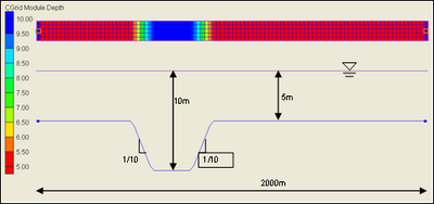
Figure33. Configuration for channel infilling tests
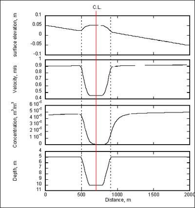
| Figure34. | Surface elevation, current velocity, and concentration calculated by AD formulation with Lund-CIRP formula |
Results of the channel infilling simulation are shown in Figure 35 (AD) and Figure 36 (TL). The AD formulation reproduces general channel deformation processes such as bank encroachment and infilling. On the other hand, the TL-model is inadequate, being capable of producing only channel bank encroachment and channel migration, but not channel infilling. Bank encroachment arises primarily from bed load transport and channel infilling primarily from suspended load transport. Thus, accurate calculation of suspended load as through an AD formulation is essential for simulating the channel infilling process.
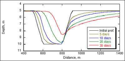
Figure35. Channel profile change by AD formulation, grain size = 0.2 mm
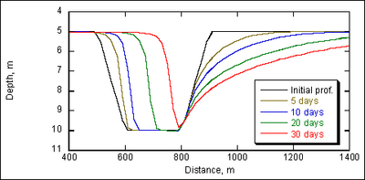
Figure36. Channel profile change by TL formulation, grain size = 0.2 mm
Figure 37 compares the channel shapes after 10 days of simulation time. Because the both simulations apply the same transport rate formula (Lund-CIRP formula), the total amount of sediment transported into the channel is almost identical, but the resultant channel shape is different. The reason for the difference is that the AD formulation calculates the advection and diffusion of suspended sediment, which the TL formulation neglects.
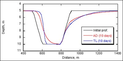
Figure37. Channel shape comparison between AD and TL formulations, grain size = 0.2 mm, 10-day simulation time
Figures 38 and 39 show the results of channel deformation for sediment grain size of 0.4 mm. In this situation, bed load transport becomes dominant as compared to the case of 0.2-mm sand grains, and the calculated channel shape is almost identical between AD and TL formulations.
In summary, if suspended load is dominant, the AD formulation can more accurately describe channel infilling, whereas if bed load is dominant, a TL formulation might be more accurate and is more efficient in terms of the allowable morphology time step. Also, from the point of view of computational costs, a TL formulation is more efficient than the AD. In the CMS-M2D system, therefore, users can select a sediment transport formulation depending on the situation. In particular, in preliminary runs, a TL formula might be selected, with the final production runs switching to an AD formulation.
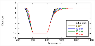
Figure38. Channel profile change by AD formulation, grain size = 0.4 mm

Figure39. Channel profile change by TL formulation, grain size = 0.4 mm
Ocean City Inlet, MD
Ocean City Inlet is a dual-jettied Federal inlet located on the coast of the Delmarva Peninsula. In August 1933, the inlet was opened as a breach in Fenwick (barrier) Island, and jetties were soon constructed to stabilize the entrance. Dean and Perlin (1977) discuss coastal and inlet processes at the site. For the present example, a December 1992 northeaster was selected to simulate hydrodynamic and sediment transport processes during a severe storm.
The example of Ocean City Inlet is provided to demonstrate the following capabilities of the CMS:
Model Steering: coupling between CMS-M2D and STWAVE
CMS-M2D forcing: extraction of boundary conditions from a regional model
Sediment transport: application of the AD transport equation.
CMS-M2D and STWAVE grids were developed for the Ocean City Inlet system so that interaction between tidal, wave, and morphology change processes could be calculated. The CMS-M2D computational domain with bathymetry and grid is shown in Figure 40. The corresponding STWAVE domain (Figure 41) is slightly larger than the CMS-M2D domain in the Atlantic Ocean, but is truncated in the bay. The STWAVE grid configuration in the Atlantic Ocean portion area is slightly larger than the CMS-M2D grid to avoid extrapolation of wave properties and radiation stresses over and near the CMS-M2D boundary. Within the bay area, the CMS-M2D grid is larger than the STWAVE grid because significant wave energy is not expected to propagate from the bay side of the inlet toward the north or south.
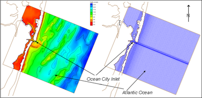
Figure40. Bathymetry and CMS-M2D computational grid for Ocean City Inlet
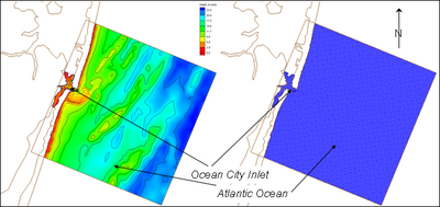
Figure41. Bathymetry and STWAVE computational grid for Ocean City Inlet
The CMS-M2D grid contains 14,886 ocean cells that have dimensions ranging from 26.5 to 127.8 m. Greatest detail is specified in the inlet and nearshore area, including the ebb shoal. The STWAVE grid contains 81,102 computational cells having dimensions of 44.9 m on each side.
For simulation of the December 1992 northeaster, a regional ADCIRC solution was available that could be applied as CMS-M2D boundary forcing. Simulation of the storm started on 8 December 1992 and ran for 8 days. The ADCIRC domain (Figure 42) is large enough to represent the storm surge propagation. Therefore, by applying the ADCIRC solution to force CMS-M2D at its ocean and bay boundaries, temporal and spatial variations in the sea surface owing to the combined wind, atmospheric pressure, and tidal forcing were preserved. An example of the spatial distribution in water-surface elevation is shown in Figure 43, during the peak surge along the Maryland coast.
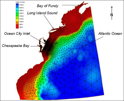
Figure42. Regional ADCIRC mesh and bathymetry for Maryland coast
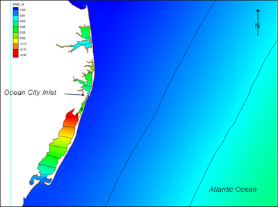
Figure43. Calculated peak water-surface elevation along Maryland coast for December 1992 storm
The 8-day CMS-M2D simulation was forced with water-surface elevation values along the ocean boundary and bay boundaries extracted from the regional ADCIRC solution for the December 1992 storm. A ramp duration of 0.5 day was specified. Wave properties at 1-hr intervals were obtained from measurements and applied as input to STWAVE. The steering interval was specified to be 1 hr. Sediment transport was computed by the AD equation with the Lund-CIRP profile option. The advection-diffusion equation was solved every 10 s and the morphologic time step was 0.25 hr.
An example of the current field during strong storm forcing is shown in Figure 44, when the surge level was 1.06 m, offshore wave conditions were height of 4.8 m, period of 14 s, and direction of 62 deg south of east. The velocity field shows a strong current generated along the outer edge of the ebb shoal from wave shoaling and breaking. A well-developed longshore current is directed toward the north.
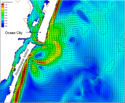
Figure44. Calculated velocity field at Ocean City Inlet during 4.8 m wave condition, December 1992 storm
A time series of current fields at 10-hr intervals is shown in Figure 45. The starting image at hour 60 corresponds to 10 December 1992 at noon. In this series of plots, changes in strength, pattern, and direction of the currents are responses to the temporal and spatial properties of the waves and to a lesser extent, the storm surge. Initially, waves propagate from the south east and drive a north-directed longshore current (through hour 90). As the wave direction rotates over the duration of the storm, the north-directed longshore current becomes weaker (hours 90–110) then turns toward the south for the remainder of the storm. Over the duration of the storm, waves reaching the ebb shoal drive currents toward the north on the northern outer portion of the shoal and toward the south and shoreward on the southern outer portion of the shoal.
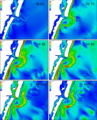
| Figure45. | Calculated velocity fields at 10-hr intervals at Ocean City Inlet, December 1992 storm
Figure 45 (continued). Calculated velocity fields at 10-hr intervals at Ocean City Inlet, December 1992 storm Morphology change calculated for the storm is evident in the inlet entrance. Figure 46 shows the initial bathymetry at the start of the simulation (hour 0), bathymetry after the longshore current has been directed northward (hour 100), and bathymetry at the end of the simulation (hour 180) during which the longshore current was directed toward the south for about the last 80 hr. Initially, the scour hole located at the inlet entrance is deepest. After 100 hr of simulation, some infilling of the scour hole had taken place with material transported from the south. After 180 hr of simulation, the scour hole had continued to fill with sediment transported from the north, which also steepened the northern flank of the scour hole (contours become slightly closer together). 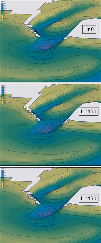 Figure46. Calculated depth at Ocean City Inlet, December 1992 storm Depth change at the inlet and ebb shoal after 100 and 180 hr of simulation is shown in Figure 47. Red and yellow denote accretion, and blue denotes erosion. The most significant changes in morphology are deposition at the inlet entrance, scour off of the tip of the north jetty, and alternating bands of accretion and erosion around the outer areas of the ebb shoal. 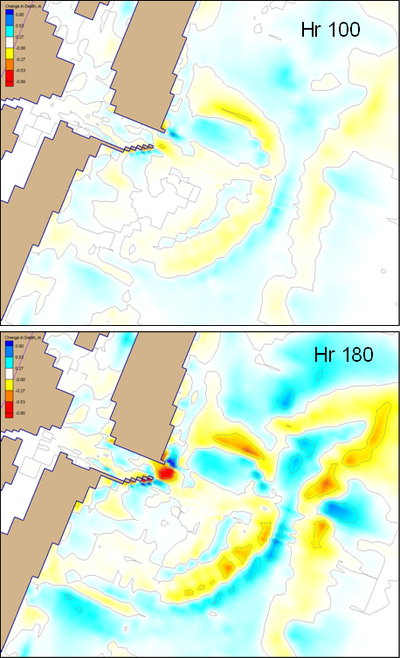 Figure47. Calculated depth change at Ocean City Inlet, December 1992 storm Sebastian Inlet, FLSebastian Inlet is on the south-central east coast of Florida and connects the Atlantic Ocean to the Indian River Lagoon. In 1927, deepening of the inlet that began in 1924 was accomplished by blasting of limestone rock. At present, most of the inlet throat is comprised of hard substrate. In addition, rock outcrops are present in the nearshore at and directly south of the inlet. Figure 48 is an image showing the inlet and extent of hard bottom. Because of the significant rock exposure, Sebastian Inlet was selected as a location to demonstrate the CMS featuring the hard-bottom capability. Bathymetry data, information on hard-bottom coverage, and forcing data (water-surface elevation and wave properties) were provided by Dr. Gary A. Zarillo, Florida Institute of Technology. 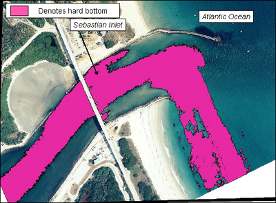
The example of Sebastian Inlet is provided to demonstrate the following capabilities of the CMS:
CMS-M2D and STWAVE grids were developed for Sebastian Inlet so that interaction between tidal, wave, and morphology change processes could be calculated. The CMS-M2D computational domain with bathymetry and grid are shown in Figure 49, and the corresponding STWAVE bathymetry and domain are shown in Figure 50. The STWAVE domain in the Atlantic Ocean portion of the grid is slightly larger than the CMS-M2D grid to avoid extrapolation of wave properties and radiation stresses over and near the CMS-M2D boundary. Within the Indian River Lagoon, the CMS-M2D grid is larger than the STWAVE grid because significant wave energy is not expected to propagate from the bay side of the inlet toward the north or south. In addition, gauge data for water-surface elevation forcing was available at the north and south lagoon extents. 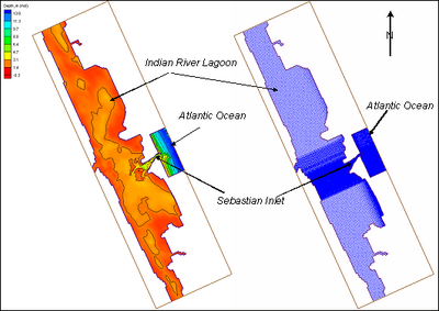 Figure49. Bathymetry and CMS-M2D computational grid for Sebastian Inlet 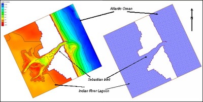 Figure50. Bathymetry and STWAVE computational grid for Sebastian Inlet The CMS-M2D grid contains 18,762 ocean cells, which have dimensions ranging from 9.6 to 99.9 m. Greatest detail is specified in the inlet and nearshore (Figure 51). Hard-bottom cells (Figure 52) were specified by overlaying the aerial photograph denoting hard-bottom areas (Figure 48) onto the CMS-M2D computational grid and assigning cells that had at least 50 percent coverage of hard bottom as non-erodible. Depth of non-erodible substrate for the hard-bottom cells was specified to be the ambient depth. The STWAVE grid contains 24,095 computational cells having dimensions of 20 m on each side. 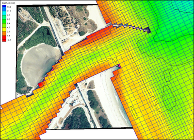
A 15-day simulation was conducted with water-surface elevation forcing along the ocean boundary and along the northern and southern boundaries located in the Indian River Lagoon. Time series for these three boundaries were obtained from hourly measurements taken from 1 January to 15 January 1997. Daily wave input to STWAVE was also obtained from measurements for the same time period. The steering interval was specified to be 6 hr. Sediment transport options included application of the Lund-CIRP total load formula with a sediment transport time step of 120 s and a morphologic time step of 0.4 hr. Suspended load and bed load scaling factors were each specified as 0.1. 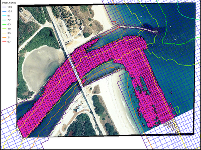
Representative ebb and flood currents calculated for Sebastian Inlet are shown in Figure 53. During ebb and flood, the strongest currents are in the center of the inlet throat and overlying hard substrate. Calculated change in depth over the simulation interval is shown in Figure 54, together with the location of hard-bottom cells denoted by triangles. In the inlet throat, deposition takes place along the southern extent of the hard-bottom cells and erosion takes place between this area of deposition and the southern inlet wall. Erosion of hard-bottom cells below the prescribed depth of the hard substrate does not take place. Material on the outer ebb shoal has migrated shoreward in response to combined wave- and current-driven transport. 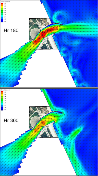
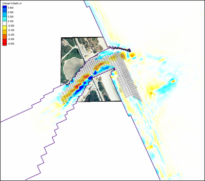 Figure54. Calculated depth change at Sebastian Inlet after 360 hr
References
Battjes, J. A. (1975). "Modeling of turbulence in the surf zone," Proceedings Symposium on Modeling Techniques, ASCE, 1,050-1,061.
Bounaiuto, F., and Militello, A. (2004). "Coupled circulation, wave, and sediment transport modeling for calculation of morphology change, Shinnecock Inlet, New York," Proceedings 8th 'International Estuarine and Coastal Modeling Conference, ASCE, 819-838.
Bretschneider, C. L. (1966). "Engineering aspects of hurricane surge," Estuary and coastline hydrodynamics, A. T. Ippen, ed., McGraw-Hill, NY, 231-256.
Brown, C. A., Kraus, N. C., and Militello A. (1995a). "Hydrodynamic modeling for assessing engineering alternatives for elevating the Kennedy Causeway, Corpus Christi, Texas," Proceedings 4th 'International Estuarine and Coastal Modeling Conference, ASCE, 681-694.
Brown, C. A., Militello, A., and Kraus, N. C. (1995b). "Hydrodynamic assessment for elevation of the JFK Causeway, Corpus Christi, Texas," Proceedings Texas Water ’95, Texas Section of the American Society of Civil Engineers, ASCE, 31-41.
Brown, C. A., Militello, A., and Kraus, N. C. (1995c). "Hydrodynamic assessment for elevation of the JFK Causeway, Corpus Christi, Texas," TAMU-CC-CBI-95-07, Conrad Blucher Institute for Surveying and Science, Texas A&M Univeristy-Corpus Christi, Corpus Christi, TX.
Butler, H. L. (1978). "Coastal flood simulation in stretched coordinates," Proceedings 16th 'Coastal Engineering Conference, ASCE, 1,030-1,048.
Camenen, B., and Larson, M. (2005). "A bedload sediment transport formula for the nearshore," Estuarine, Coastal and Shelf Science 63, 249-260.
Camenen, B., and Larson, M. (2006). "A suspended load sediment transport formula for the nearshore," Journal of Coastal Research (in review).
Charnock, H. (1955). "Wind stress on a water surface," Quarterly Journal of the Royal Meteorological Society 81, 639-640.
Cialone, M. A. (1989). "Curvilinear long wave hydrodynamic (CLHYD) model for tidal circulation and storm surge propagation," Proceedings 1st 'Conference on Estuarine and Coastal Modeling, ASCE, 16-26.
Dally, W. R., and Brown, C. A. (1995). "A modeling investigation of the breaking wave roller with application to cross-shore currents," Journal of Geophysical Research 100(C12), 24,873-24,883.
Dally, W. R., Dean, R. G., and Dalrymple, R. A. (1985). "Wave height variation across beaches of arbitrary profile," Journal of Geophysical Research 90(C6), 11,917-11,927.
Dally, W. R., and Osiecki, D. A. (1994). "The role of rollers in surf zone currents," Proceedings 24th 'Coastal Engineering Conference, ASCE, 1,895-1,905.
Dean, R. G., and Perlin, M. (1977). "Coastal engineering study of Ocean City Inlet, Maryland," Proceedings Coastal Sediments ’77, ASCE, 520-542.
Eckart, C. (1952). "The propagation of waves from deep to shallow water," in Gravity waves, National Bureau of Standards, Circular No. 521, 165-173.
Elder, J. W. (1959). "The dispersion of marked fluid in turbulent shear flow," Journal of Fluid Mechanics 5, 544-560.
Falconer, R. A. (1980). "Modelling of planform influence on circulation in harbors," Proceedings 17th 'Coastal Engineering Conference, ASCE, 2,726-2,744.
Flather, R. A., and Heaps, N. S. (1975). "Tidal computations for Morecambe Bay," Geophysical Journal of the Royal Astronomical Society London A210, 423-436.
Hanson, H. (1989). "GENESIS - A generalized shoreline change numerical model," Journal of Coastal Research 5(1), 1-27.
Hanson, H. and Kraus, N.C. (1985). "Seawall constraint in the shoreline numerical model," Journal of Waterway, Port, Coastal and Ocean Engineering 111(6), 1079 1083.
Hanson, H. and Kraus, N. C. (1986). "Seawall boundary condition in numerical models of shoreline change," Technical Report CERC 86 3, U.S. Army Engineer Waterways Experiment Station, Coastal Engineering Research Center, Vicksburg, MS.
Hanson, H., and Kraus, N. C. (1989). "GENESIS: Generalized model for simulating shoreline change. Report 1: Technical reference," Technical Report CERC-89-19, U.S. Army Engineer Waterways Experiment Station, Coastal Engineering Research Center, Vicksburg, MS.
Hanson, H., and Militello, A. (2005). "Representation of non-erodible (hard) bottom in two-dimensional morphology change models," Coastal and Hydraulic Engineering Technical Note ERDC/CHL CHETN-IV-63, U.S. Army Engineer Research and Development Center, Vicksburg, MS.
Hsu, S. A. (1988). Coastal meteorology. Academic Press, San Diego, CA.
Irie, I., Kuriyama, Y., and Tagawa, M. (1985). "Prediction of sea bed topography by combination of physical and numerical model," Proceedings Coastal Engineering Conference 32, Japan Society of Civil Engineers, 345-350, (in Japanese).
Kraus, N. C. (2006). "Coastal inlet functional design: Anticipating morphologic response, Proceedings Coastal Dynamics ’05, ASCE, in press.
Kraus, N. C., and Larson, M. (1991). "NMLONG: Numerical model for simulating the longshore current: Report 1: Model development and tests," Dredging Research Report DRP-91-1, U.S. Army Engineer Waterways Experiment Station, Vicksburg, MS.
Kraus, N. C., and Militello, A. (1996). "Hydraulic feasibility of the proposed Southwest Cut, East Matagorda Bay, Texas," TAMU-CC-CBI-96-03, Conrad Blucher Institute for Surveying and Science, Texas A&M University-Corpus Christi, Corpus Christi, TX.
Kraus, N. C., and Militello, A. (1999). "Hydraulic study of multiple inlet system: East Matagorda Bay, Texas," Journal of Hydraulic Engineering 125, 3, 224-232.
Kraus, N. C., Arden, H. T., and Simpson, D. P., eds. (2002). "Study of navigation channel feasibility, Willapa Bay, Washington: Report 2: Entrance channel monitoring and study of Bay Center entrance channel," ERDC/CHL TR-00-6, U.S. Army Research and Development Center, Coastal and Hydraulics Laboratory, Vicksburg, MS.
Larson, M., and Kraus, N. C. (1989). "SBEACH: Numerical model for simulating storm-induced beach change: Report 1: Empirical foundation and model development," Technical Report CERC-89-9, U.S. Army Engineer Waterways Experiment Station, Coastal Engineering Research Center, Vicksburg, MS.
Larson, M., and Kraus, N. C. (2002). "NMLONG: Numerical Model for Simulating Longshore Current: Report 2: Wave-current interaction, roller modeling, and validation of model enhancements," Technical Report ERDC/CHL TR-02-22, U.S. Army Engineer Research and Development Center, Vicksburg, MS.
Le Provost, C., Genco, M. L., Lyard, F., Vincent, P., and Canceill, P. (1994). "Spectroscopy of the world ocean tides from a hydrodynamic finite element model," Journal of Geophysical Research 99(C12), 24,777-24,797.
Lin, L., Kraus, N. C, and Barcak, R. G. (2004). "Modeling sediment transport at the Mouth of the Colorado River, Texas," Proceedings 8th 'International Estuarine and Coastal Modeling Conference, ASCE, 988-1006.
Lin, L., Mase, H., Yamada, F., and Demirbilek, Z. (2006). "Wave-Action Balance Equation Diffraction (WABED) Model, Part 1: Tests of Wave Diffraction and Reflection at Inlets," Coastal and Hydraulic Engineering Technical Note ERDC/CHL CHETN-III-73, U.S. Army Corps of Engineer Research and Development Center, Vicksburg, MS.
Luettich, R. A., Westerink, J. J., and Scheffner, N. W. (1992). "ADCIRC: An advanced three-dimensional circulation model for shelves, coasts, and estuaries; Report 1: Theory and methodology of ADCIRC-2DDI and ADCIRC-3DL," Dredging Research Report DRP-92-6, U.S. Army Engineer Waterways Experiment Station, Vicksburg, MS.
Madsen, O. S., and Grant, W. D. (1976). "Sediment transport in the coastal environment," Technical Report 209, M.I.T., Cambridge, MA, 105 pp.
Mase, H. (2001). "Multi-directional random wave transformation model based on energy balance equation," Coastal Engineering Journal 43(4), 317-337.
Mase, H., and Kitano, T. (2000). "Spectrum-based prediction model for random wave transformation over arbitrary bottom topography," Coastal Engineering Journal 42(1), 111-151.
Mase, H., Oki, K., Hedges, T., and Li, H. J. (2005). "Extended energy-balance-equation wave model for multidirectional random wave transformation," Ocean Engineering 32, 961-985.
Militello, A. (1998). Hydrodynamics of wind-dominated, shallow embayments. Ph.D. dissertation, Division of Marine and Enviromental Systems, Florida Institute of Technology, Melbourne, FL.
Militello, A. (2000). "Hydrodynamic modeling of a sea-breeze dominated shallow embayment, Baffin Bay, Texas," Proceedings 6th 'International Estuarine and Coastal Modeling Conference, ASCE, 795-810.
Militello, A. (2002). "Willapa entrance and Bay Center modeling," in "Study of navigation channel feasibility, Willapa Bay, Report 2," N. C. Kraus, H. T. Arden, and D. P. Simpson, eds. Technical Report ERDC-CHL-TR-00-6, U.S. Army Engineer Research and Development Center, Vicksburg, MS.
Militello, A., and Kraus, N. C. (1998). "Numerical simulation of hydrodynamics for proposed inlet, East Matagorda Bay, Texas," Proceedings 5th 'International Estuarine and Coastal Modeling Conference, ASCE, 805-818.
Militello, A., and Kraus, N. C. (2001). "Generation of harmonics by sea breeze in nontidal water bodies," Journal of Physical Oceanography 31(6), 1639-1647.
Militello, A., and Kraus, N. C. (2003). "Numerical simulation of sediment pathways at an idealized inlet and ebb shoal," Coastal Sediments 2003, CD ROM: Numerical simulation of sediment pathways at an id.pdf.
Militello, A., Parry, R. M., and Arden, H. T. (2003). "Numerical simulation of navigation channel infilling, Bay Center, Washington," Proceedings Dredging 2002 Conference, ASCE, CD-ROM 40680-034, ISBN 0-7844-0680-4.
Militello, A., Reed, C. W., Zundel, A. K., and Kraus, N. C. (2004). "Two-dimensional depth-averaged circulation model M2D: Version 2.0, Report 1: Documentation and user’s guide," ERDC/CHL TR-04-02, U.S. Army Engineer Research and Development Center, Vicksburg, MS.
Militello, A., and Zundel, A. K. (2002a). "Automated coupling of regional and local circulation models through boundary condition specification," Proceedings 5th 'International Conference on Hydroinformatics, International Association of Hydraulic Research IWA Publishing, London, 156-161.
Militello, A., and Zundel, A. K. (2002b). "Coupling of regional and local circulation models ADCIRC and M2D," Coastal and Hydraulics Engineering Technical Note CHETN-IV-42, U.S. Army Engineer Research and Development Center, Vicksburg, MS.
Militello, A., and Zundel, A. K. (2003). "SMS Steering Module for coupling waves and currents, 2. M2D and STWAVE," Coastal and Hydraulics Engineering Technical Note ERDC/CHL CHETN-IV-60, U.S. Army Engineer Research and Development Center, Vicksburg, MS.
Mukai, A. Y., Westerink, J. J., Luettich, R. A., Jr., and Mark, D. (2002). "Eastcoast 2001, A Tidal Constituent Database for Western North Atlantic, Gulf of Mexico, and Caribbean Sea," Coastal Inlets Research Program, Technical Report ERDC/CHL-TR-02-24, U.S. Army Engineer Research and Development Center, Vicksburg, MS.
Nielsen, P. (1992). Coastal bottom boundary layers and sediment transport, World Scientific, New Jersey, 324 pp.
Nishimura, H. (1988). "Computation of neasrshore current." In Nearshore dynamics and coastal processes, K. Horikawa, ed., University of Tokyo Press, Tokyo, Japan, 271-291.
Putrevu, U., and Svendsen, I. A. (1992). "A mixing mechanism in the nearshore region," Proceedings 23rd 'International Coastal Engineering Conference, ASCE, 2,578-2,771.
Reed, C. W., and Militello, A. (2005). "Wave-adjusted boundary condition for longshore current in finite-volume circulation models," Ocean Engineering 32, 2121-2134.
Reid, R. O., and Bodine, B. R. (1968). "Numerical model for storm surges in Galveston Bay," Journal of the Waterways and Harbors Division, 94(WW1), 33-57.
Richtmyer, R. D., and Morton, K. W. (1967). Difference methods for initial-value problems. Interscience Publishers, NY, 405 pp.
Roache, P. J. (1976). Computational fluid dynamics. Hermosa Publishers, Albuquerque, NM, 446 pp.
Saville, T., Jr. (1953). "Wind setup and waves in shallow water," Beach Erosion Board Technical Memorandum No. 27, U.S Army Corps of Engineers.
Schureman, P. (1924). "A manual of the harmonic analysis and prediction of tides," U.S. Coast and Geodetic Survey, Special Publication 98, 426 pp.
Shore protection manual (1984). 4th ed., 2 Vol., U.S. Army Engineer Waterways Experiment Station, U.S. Government Printing Office, Washington, DC.
Smith, J. M., Larson, M., and Kraus, N. C. (1993). "Longshore current on a barred beach: Field measurements and calculation," Journal of Geophysical Research 98(C12), 22,717-22,731.
Smith, J. M., Resio, D. T., and Zundel, A. K. (1999). "STWAVE: STeady-state spectral WAVE model, Report 1: User’s manual for STWAVE Version 2.0," Instructional Report CHL-99-1, U.S. Army Engineer Waterways Experiment Station, Vicksburg, MS.
Smith, J. M., Sherlock, A. R., and Resio, D. T. (2001). "STWAVE: STeady-state spectral WAVE model: User’s manual for STWAVE Version 3.0," Supplemental Report ERDC/CHL SR-01-1, U.S. Army Engineer Research and Development Center, Vicksburg, MS.
Soulsby, D. H. (1997). "Dynamics of marine sands. A manual for practical applications," Thomas Telford Publications, London, England, 249 pp.
Spaulding, M. L. (1984). "A vertically averaged circulation model using boundary fitted coordinates," Journal of Physical Oceanography 14, 973-982.
Swart, D. H. (1974). "Offshore sediment transport and equilibrium beach profiles," Delft Hydraulics Laboratory Publications 131, Delft, The Netherlands, 302 pp.
van Rijn, L. (1985). "Two-dimensional vertical mathematical model for suspended sediment transport by currents and waves," Report S488-IV, Delft Hydraulics, Delft, The Netherlands.
van Rijn, L. (1993). Principles of sediment transport in rivers, estuaries, and coastal seas. Aqua Publications, Amsterdam, The Netherlands, 673 pp.
van Rijn, L. (1998). Principles of coastal morphology. Aqua Publications, Amsterdam, The Netherlands.
Visser, P. J. (1982). "Uniform longshore current measurements and calculations," Proceedings 19th 'Coastal Engineering Conference, ASCE, 2,192-2,207.
Wanstrath, J. J. (1978). "An open-coast mathemetical storm surge model with coastal flooding for Lousiana; Report 1: Theory and application," Miscellaneous Paper H-78-5, U.S. Army Engineer Waterways Experiment Station, Vicksburg, MS.
Watanabe, A. (1987). "3-dimensional numerical model of beach evolution," Proceedings Coastal Sediments ’87, ASCE, 802-817.
Wilson, K. (1966). "Bed-load transport at high shear stress," Journal of the Hydraulics Division 92(11), 49-59.
Wilson, K. (1989). "Friction of wave induced sheet flow," Coastal Engineering 12, 371-379.
Wozencraft, J. M., Lillycrop, W. J., and Kraus, N. C. (2002). "SHOALS Toolbox: Software to support visualization and analysis of large, high-density data sets," ERDC/CHL CHETN-IV-43, U.S. Army Engineer Research and Development Center, Vicksburg, MS.
Yeh, G.-T., and Chou, F.-K. (1978). "Moving boundary numerical surge model," Journal of the Waterway Port Coastal and Ocean Division 105(WW3), 247-263.
Zundel, A. K. (2000). "Surface-water Modeling System reference manual," Brigham Young University, Environmental Modeling Research Laboratory, Provo, UT.
Appendix A | |||||||||||||||||||||||||||||||||||||||||||||||||||||||||||||||||||||||||||||||||||||||||||||||||||||||||||||||||||||||||||||||||||||||||||||||||||||||||||||
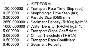
| Figure A11. | Example sedparams.dat input file for Watanabe total load formulation |
An example sedparams.dat file for the Lund-CIRP total load formulation option is provided in Figure A12. The first line contains a value of 2, which informs CMS-M2D that the Lund-CIRP total load formulation is to be applied. The remaining lines contain the input options and parameters required by the Lund-CIRP formulation and morphology change calculations.
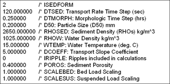
| Figure A12. | Example sedparams.dat input file for Lund-CIRP total load formulation |
An example sedparams.dat file for the AD equation option is provided in Figure A13. The first line contains a value of 3, which informs CMS-M2D that the AD equation is to be applied. The remaining lines contain the input options and parameters required by the AD equation and morphology change calculations. In this example, a value of 3 for the suspended concentration profile denotes that the Lund-CIRP formulation will be applied. A value of 1 for the suspended concentration profile denotes that the exponential model will be applied and a value of 2 denotes that the van Rijn model will be applied.
Figure A13. Example sedparams.dat input file for AD equation
An example portion of a time series numerical station output file is shown in Figure A14, in which five cells were selected for output. The cell numbers for the five cells are 1, 2, 3, 4, and 5. Time is elapsed time in days since the beginning of the simulation.
Figure A14. Example time series numerical station output file
Example portions of global elevation and velocity files are shown in Figures A15 and A16, respectively. In these examples, the time of the output is 5.6 hr after the beginning of the simulation. Coordinates of cell positions are given in the first two columns in order of ascending cell number. Cell coordinates are those specified in the grid file in the x-dist and y-dist columns (grid not shown for these global output examples). Water level is given in meters (third column), following cell coordinates; x- and y-components of velocity are given in meters per second (third and fourth columns, respectively). If multiple times of global values are written, they are successively appended at the end of the file with no lines between snapshots. Global depth files have the same format as global elevation files, and global transport rate files have the same format as global velocity files, thus, examples portions of global depth and global transport rate files are not shown.
Figure A15. Example global elevation output file
Figure A16. Example global velocity output file
Appendix B
M2D Citations
This appendix contains a listing of publications known to the authors to date that document M2D and its applications. Citations are listed in reverse chronological order.
Buttolph, A. M., Reed, C. W., Kraus, N. C., Ono, N., Larson, M., Camenen, B., Hanson, H., Wamsley, T., and Zundel, A. K. (2006). "Two-dimensional depth-averaged circulation model CMS-M2D: Version 3.0, Report 2: Sediment Transport and Morphology Change," ERDC/CHL TR-06-__, U.S. Army Engineer Research and Development Center, Vicksburg, MS (this volume).
Lin, L., Mase, H., Yamada, F., and Demirbilek, Z. (2006). "Wave-Action Balance Equation Diffraction (WABED) Model; Part 1: Tests of wave diffraction and reflection at inlets," Coastal Inlet Research Program Technical Note ERDC/CHL CHETN-III-73, U.S. Army Engineer Research and Development Center, Vicksburg, MS.
Offshore & Coastal Technologies, Inc. (2005). "An assessment of jetty shortening alternatives for Goldsmith Inlet, bay and adjacent shorelines," Project report for Town of Southold, NY, 66 pp.
Offshore & Coastal Technologies, Inc. (2005). "Ocean City hot spot study: Reassessment of design criteria and approaches," Engineering Appendix for U.S. Army Engineer District, Baltimore, General Re-evaluation Report, 109 pp.
Reed, C. W., and Militello, A. (2005). "Wave-adjusted boundary condition for longshore current in finite-volume circulation models," Ocean Engineering 32, 2121-2134
Hanson, H., and Militello, A. (2005). "Representation of non-erodible (hard) bottom in two-dimensional morphology change models," Coastal and Hydraulics Engineering Technical Note ERDC/CHL CHETN-IV-63, U.S. Army Engineer Research and Development Center, Vicksburg, MS.
Bounaiuto, F., and Militello, A. (2004). "Coupled circulation, wave, and sediment transport modeling for calculation of morphology change, Shinnecock Inlet, New York," Proceedings 8th 'International Estuarine and Coastal Modeling Conference, ASCE, 819-838.
Lin, L., Kraus, N. C, and Barcak, R. G. (2004). "Modeling sediment transport at the Mouth of the Colorado River, Texas," Proceedings 8th 'International Estuarine and Coastal Modeling Conference, ASCE, 988-1006.
Militello, A., Reed, C. W., Zundel, A. K., and Kraus, N. C. (2004). "Two-dimensional depth-averaged circulation model M2D: Version 2.0, Report 1: Documentation and user’s guide," ERDC/CHL TR-04-02, U.S. Army Engineer Research and Development Center, Vicksburg, MS.
Militello, A., and Zundel, A. K. (2003) "SMS Steering Module for coupling waves and currents, 2. M2D and STWAVE," Coastal and Hydraulic Engineering Technical Note ERDC/CHL CHETN-IV-60, U.S. Army Engineer Research and Development Center, Vicksburg, MS.
Militello, A., and Kraus, N. C. (2003). "Numerical simulation of sediment pathways at an idealized inlet and ebb shoal," Coastal Sediments 2003, CD ROM: Numerical simulation of sediment pathways at an id.pdf.
Militello, A., Parry, R. M., and Arden, H. T. (2003). "Numerical simulation of navigation channel infilling, Bay Center, Washington," Proceedings Dredging 2002 Conference, ASCE, CD ROM 40680-034-003, ISBN 0-7844-0680-4.
Militello, A., and Zundel, A. K. (2002). "Coupling of regional and local circulation models ADCIRC and M2D," Coastal and Hydraulics Engineering Technical Note ERDC/CHL CHETN-IV-42, U.S. Army Engineer Research and Development Center, Vicksburg, MS.
Militello, A., and Zundel, A. K. (2002). "Automated coupling of regional and local circulation models through boundary condition specification," Proceedings 5th 'International Conference on Hydroinformatics, International Association of Hydraulic Research, IWA Publishing, London, 156-161.
Militello, A. (2002). "Willapa entrance and Bay Center modeling," in "Study of navigation channel feasibility, Willapa Bay, Report 2," N. C. Kraus, H. T. Arden, and D. P. Simpson, eds. Technical Report ERDC-CHL-TR-00-6, U.S. Army Engineer Research and Development Center, Vicksburg, MS.
Militello, A., and Kraus, N. C. (2001). "Generation of harmonics by sea breeze in nontidal water bodies," Journal of Physical Oceanography 31(6), 1,639-1,647.
Militello, A. (2000). "Hydrodynamic modeling of a sea-breeze dominated shallow embayment, Baffin Bay, Texas," Proceedings 6th 'International Estuarine and Coastal Modeling Conference, ASCE, 795-810.
Kraus, N. C., and Militello, A. (1999). "Hydraulic study of multiple inlet system: East Matagorda Bay, Texas," Journal of Hydraulic Engineering 125(3), 224-232.
Militello, A., and Kraus, N. C. (1998). "Numerical simulation of hydrodynamics for proposed inlet, East Matagorda Bay, Texas," Proceedings 5th 'International Estuarine and Coastal Modeling Conference, ASCE, 805-818.
Militello, A. (1998). Hydrodynamics of wind-dominated, shallow embayments. Ph.D. dissertation, Division of Marine and Enviromental Systems, Florida Institute of Technology, Melbourne, FL.
Brown, C. A., and Militello, A. (1997). "Packery Channel feasibility study: Circulation and water level; Report 2 of a two-part series," TAMU-CC-CBI-96-07, Conrad Blucher Institute for Surveying and Science, Texas A&M University-Corpus Christi, Corpus Christi, TX.
Kraus, N. C., and Militello, A. (1996). "Hydraulic feasibility of the proposed Southwest Cut, East Matagorda Bay, Texas," TAMU-CC-CBI-96-03, Conrad Blucher Institute for Surveying and Science, Texas A&M University-Corpus Christi, Corpus Christi, TX.
Militello, A., and Kraus, N. C. (1995). "Investigation of the current and sediment movement in the Lower Laguna Madre, Texas, and implications for dredging in the Gulf Intracoastal Waterway," Proceedings Western Dredging Association 16th 'Technical Conference, Center for Dredging Studies, Texas A&M University, College Station, TX, 143-162.
Brown, C. A., Kraus, N. C., and Militello A. (1995). "Hydrodynamic modeling for assessing engineering alternatives for elevating the Kennedy Causeway, Corpus Christi, Texas," Proceedings 4th 'International Estuarine and Coastal Modeling Conference, ASCE, 681-694.
Brown, C. A., Militello, A., and Kraus, N. C. (1995). "Hydrodynamic assessment for elevation of the JFK Causeway, Corpus Christi, Texas," Proceedings Texas Water ’95, Texas Section of the American Society of Civil Engineers, ASCE Press, NY, 31-41.
Brown, C. A., Militello, A., and Kraus, N. C. (1995). "Hydrodynamic assessment for elevation of the JFK Causeway, Corpus Christi, Texas," TAMU-CC-CBI-95-07, Conrad Blucher Institute for Surveying and Science, Texas A&M Univeristy-Corpus Christi, Corpus Christi, TX.
Militello, A., and Kraus, N. C. (1995). "Numerical simulation of the circulation in the Lower Laguna Madre, Texas, and implications for dredging of the Gulf Intracoastal Waterway," Estuarine Research Federation 13th 'Biennial International Conference, Abstracts, 88.
Militello, A., and Kraus, N. C. (1994). "Reconnaissance investigation of the current and sediment movement in the Lower Laguna Madre between Port Isabel and Port Mansfield, Texas," TAMU-CC-CBI-94-04, Conrad Blucher Institute for Surveying and Science, Texas A&M University-Corpus Christi, Corpus Christi, TX.
Appendix C
Slosh Tests
This appendix describes the performance of CMS-M2D for slosh tests. This set of numerical integrity tests evaluates mass conservation and numerical damping properties of the model. Approximations to the full equations of motion truncate terms to some order in a manner that depends on the numerical solution method. Truncation of terms is known to introduce numerical viscosity (Roache 1976),[1] which is manifested as damping of a signal. The slosh test provides a means of examining the damping properties of numerical computation methods. In a slosh test, the initial condition of a tilted water surface is imposed, and the basin is allowed to freely propagate the resulting wave through reflection at both ends. External forcing and bottom frictional stress are set to zero so that there is no masking of the free-surface oscillations. Time-series of water elevation over the duration of the simulation exhibit model damping properties. Tests described here were patterned after those by Cialone (1989).
The slosh test was performed to examine damping properties and mass conservation for two grid configurations. Both grid configurations were rectangular, with the grid being longer parallel to the x-axis than parallel to the y-axis. A test consisted of applying a tilted water surface as the initial condition, where the direction of tilt was parallel to the x-axis. The initial deviation from still-water depth was symmetric about the channel center and increased or decreased sinusoidally along the main channel axis (Figure C1).
No variation in water level was specified across the width (parallel to the y-axis) of the channel. Initial current velocity was set to zero, and no boundary forcing, bottom friction, or wind stress was applied. The Coriolis term and lateral mixing were set to zero. Simulation duration was set to 30 days (720 hr) and the time step was set to 5 s. General grid configurations and inclusion of advective terms are given in Table C1. Conducting identical tests with and without inclusion of the advective terms allows isolation of their contribution to damping and mass conservation.
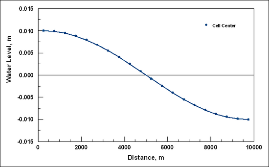
Figure C1. Slosh test initial condition
| Table C Slosh Test Configurations | ||
| Test | Bottom | Advection |
| 1 | Flat | No |
| 2 | Flat | Yes |
| 3 | Sloped | No |
| 4 | Sloped | Yes |
Mass conservation was calculated as percent change in water volume over the numerical grid between time t = 0 and the end of the simulation period. Percent change in water volume![]() was calculated as:
was calculated as:
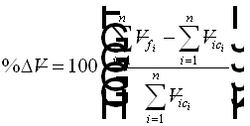
|
(C1) |
where![]() is the final volume,
is the final volume,![]() is the initial volume, the subscript i indicates cell number, and n is the total number of cells in the grid.
is the initial volume, the subscript i indicates cell number, and n is the total number of cells in the grid.
Tests 1 and 2 were conducted to evaluate damping and mass conservation of the model for a flat-bottomed, constant-spaced grid, with and without the advective terms included in the calculations, respectively. Grid configurations and numerical parameters for Tests 1 and 2 are given in Table C2, and the grid is shown in Figure C2. Tests 1 and 2 resulted in 5 ´ 10-6 and 1 ´ 10-5 percent changes in volume, respectively.
| Table C2 Slosh Test Grid Configurations and Numerical Parameters for Tests 1 and 2 | ||
| Numerical Parameter | Value | |
| D'''s''', m | 500 | |
| D'''t''', s | 5 | |
| h, 'm' | 10 | |
| Length, m | 10,000 | |
| Width, m | 2,500 | |
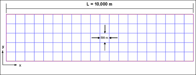
Figure C2. Computational grid for Tests 1 and 2
Damping properties for Tests 1 and 2 are shown by time series of water level in Figures C3 and C4, respectively. Water levels shown for each plot were taken 0.5 Dx from the boundary and centered with respect to channel width. Time series shown for all other tests are also taken at the same cell. Axis breaks (x‑axis) were inserted into the plots so that time series at the beginning and ending portions of the simulations could be easily viewed. Test 1 does not exhibit damping over the duration of the simulation. Weak nonlinear motion owes to the nonlinear form of the continuity equation. Test 2 exhibits weak damping over the 1-month simulation. Development of nonlinearities is slightly stronger than for Test 1 owing to the contribution by the advective terms. Tests 1 and 2 were repeated with an initial surface deviation 10 times smaller than described here (results not shown). Motion induced by this smaller water-surface deviation was not sufficient to develop nonlinearities and the resulting slosh motion for both cases (with and without advection) showed no variation in peak water level, and no damping was exhibited.
The fundamental seiche period for a rectangular basin is given by:

|
(C2) |
where l is the length of the basin. For a wave traveling parallel to the x-axis of the slosh-test grid, T = 0.02337 day, corresponding to a frequency of 42.8 cycles/day (cpd). Spectrums of water levels shown in Figures C3 and C4 for Tests 1 and 2 are displayed in Figures C5 and C6, respectively. Peak amplitudes occur at 42.8 cpd. Small peaks (slightly visible in Figures C5 and C6) are contained in the spectra at 85.6 cpd, indicating the presence of a weak harmonic of the primary seiche frequency. These tests indicate that the discretized equations applied for calculation of water level in Tests 1 and 2 do not introduce erroneous frequencies into the solution.
Figure C3. Time series of water level for Test 1
Figure C4. Time series of water level for Test 2
Figure C5. Spectrum of water level for Test 1
Figure C6. Spectrum of water level for Test 2
Tests 3 and 4 were designed to determine how damping and mass conservation properties respond to a grid with sloped bottom and constant cell sizes. Grid configurations and numerical parameters for Tests 3 and 4 are given in Table C3 and the grid is shown in Figure C7. Changes in volume of 5 ´ 10-6 and 1 ´ 10-5 percent were calculated for Tests 3 and 4, respectively.
| Table C Slosh Test Grid Configurations and Numerical Parameters for Tests 3 and 4 | ||
| Numerical Parameter | Value | |
| D'''s''', m | 500 | |
| D'''t''', s | 5 | |
| h, 'm' | Min = 9 m, Max = 11 m, Dh /Dx = 0.0002 | |
| Length, m | 10,000 | |
| Width, m | 2,500 | |
Figure C7. Computational grid for Tests 3 and 4
Damping properties for Tests 3 and 4 are shown by time series of water level in Figures C8 and C9, respectively. Starting maximum water level for both tests was 0.01 m at 0.5Dx from the end of the grid. Test 3 does not exhibit damping over the duration of the simulation. Water levels from Test 4 are slightly damped by properties of the numerical algorithm for the advective terms. In both tests, water levels are weakly nonlinear, as described for Tests 1 and 2.
Spectrums of water levels for Tests 3 and 4 are displayed in Figures C10 and C11, respectively. Peak amplitudes occur at 42.4 cpd. Small peaks (slightly visible in Figures C5 and C6) are contained in the spectra at 84.8 cpd, indicating the presence of a weak harmonic of the primary seiche frequency. These spectra demonstrate that the discretized equations applied for calculation of water level in Tests 3 and 4 do not introduce erroneous frequencies into the solution.
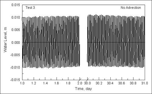 Figure C8. Time series of water level for Test 3
Figure C9. Time series of water level for Test 4
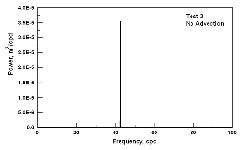 Figure C10. Spectrum of water level for Test 3
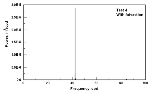 Figure C11. Spectrum of water level for Test 4
Appendix D
Wind Set Up Tests
This appendix describes tests designed to evaluate model performance under wind forcing. Two tests were performed to examine model response. The first test compares the results of numerical calculations to those of an analytical solution for a rectangular channel. The second test evaluates model response to wind forcing in a basin of arbitrary shape.
Wind set up in a rectangular channel for steady-state conditions is maintained by a balance of the pressure gradient, wind forcing, and bottom friction. For 1D flow, the momentum equation (Equation 2) can be reduced to (Bretschneider 1966)[2]:

|
(D1)
|
where Tw is the wind stress, and Tb is the bottom stress. In the absence of bottom friction, Equation D1 of Bretschneider can be rewritten as:

|
(D2)
|
where κ=3.3x10⁻⁶. The coefficient k was derived from wind and bottom-stress coefficients determined in a study of Lake Okeechobee, FL (Saville 1953). Application of Equation D2 to the present study required modification of k to be equal to the wind-stress coefficient applied in CMS-M2D, which varies with wind speed, so that analytical and numerical solutions could be compared. Integration of Equation D2 gives:

|
(D3)
|
where C is a constant of integration that is determined by the position of the channel origin if no bottom is exposed, and by the position of the water-land interface if drying has occurred. The parabolic form of Equation D3 indicates a locally wind-forced water surface in a rectangular channel does not have a linear distribution along the channel axis. Instead, the water surface will be curved, with the curvature being dependent on the channel length and depth, and the wind speed.
For comparison of the analytical and numerical solutions of Equation D2, a 1D grid was developed that had a total length of 9,500 m and was 95 cells long. Each square cell had side dimensions of 100 m. The still-water depth was set to 2 m and the time step was 10 s. The wind speed set to 10 m/s and held constant. A 10-m/s wind speed corresponds to
. Figure D1 compares water level computed analytically from Equation D2 and numerically by CMS-M2D, under steady-state conditions. The numerical solution well reproduces the steady-state, wind-induced set up and set down of the analytical solution for simulations applied to shallow water.
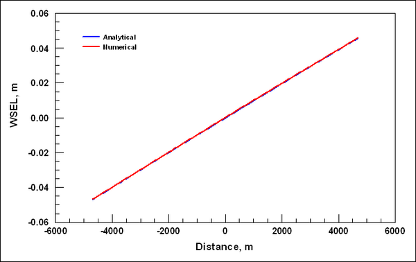
| Figure D1. | Comparison of analytical and numerical solutions of steady-state, wind-induced set up, no exposed channel bottom
|
To test the response of the model to wind forcing in a basin of arbitrary geometry, a modified version of the hourglass test developed for a curvilinear grid (Spaulding 1984) was examined. An hourglass-shaped grid was developed with constant cell-side lengths set to 500 m and an ambient depth of 5 m. The time step was set to 30 s. Two tests were performed, one for wind blowing from the west (from the negative x-axis) and the other for wind blowing from the north (from the positive y-axis). For each test, the wind was ramped up over a 24-hr interval and held constant at 10 m/s for the remainder of the 100-hr simulation.
Water-surface elevation for the west wind test is shown in Figure D2. The set up and set down are symmetric between the upper and lower portions of the grid. The water-surface elevation contours for the north wind test are shown in Figure D3. The water-surface elevation for the north wind test is equally distributed between the left and right portions of the grid. Symmetry in both tests demonstrates that there is no inconsistency in calculations at wall boundaries. The results of this test demonstrate that the model responds to wind forcing with qualitatively correct patterns of water-surface deviation. Wind set up calculated by CMS-M2D is qualitatively similar to results displayed graphically by Spaulding (1984) and by Cialone (1989).
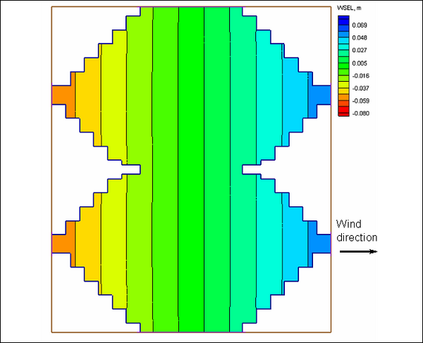
Figure D2. Water-surface elevation contours for west wind
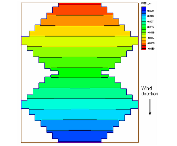
Figure D3. Water-surface elevation contours for north wind
Appendix E
Advection Test
Advective terms were examined by developing a grid with an idealized jettied inlet and displaying the current field during ebb flow. Inclusion of the advective terms in the momentum equations allows the model to properly simulate eddies and an ebb jet as the ebb flow exits the inlet. Eddies and jets will not develop without advective terms represented in the calculations.
The idealized inlet grid was specified to have a flat bottom with a still-water depth of 5 m. Inlet dimensions were 300 m wide and 800 m long. Cell-side lengths were 25 m on all sides in the inlet and nearshore areas. Cell size increased to 50 m offshore. The time step was set to 1 s. Water level was forced with a sine wave having amplitude of 0.5 m and period of 12.42 hr.
Two simulations were conducted, one without advective terms included in the computations and one with them. Figure E1 shows the current field from the test without the advective terms during the ebb tidal cycle. No eddies are present and flow exiting the inlet spreads laterally, but does not form a jet. However, with the advective terms included in the computations (Figure E2), a well-developed ebb jet is formed and eddies are present on each side of the jet. The ebb jet and eddies are symmetrical about the axis of the inlet, demonstrating that there is no directional bias in the advection algorithm.
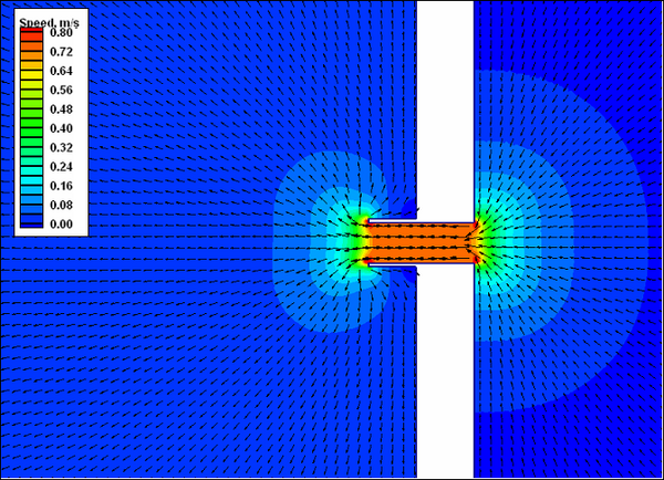
Figure E1. Ebb current field for advection test, no advective terms
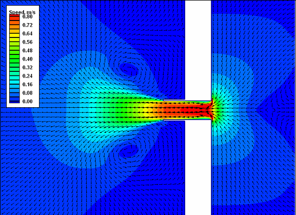
Figure E2. Ebb current field for advection test, with advective terms
Appendix F
Wetting and Drying Tests
Tests were performed on a sloped-bottom grid to determine the stability properties of the wetting and drying algorithms. One- and two-dimensional tests were conducted to demonstrate the behavior of the flooding and drying algorithms under different sources of hydrodynamic forcing and basin geometries. A list and short description of the tests are given in Table F1. Comprehensive descriptions and model results are provided for specific tests.
| Table F1 List and Description of Flooding and Drying Tests | ||
| Test Number | Title | Description |
| 1 | Channel with sloping bottom | Test wetting and drying of a 1D canal forced by time-varying wind. |
| 2 | Depression in a square grid | Test stability for wetting dry cells surrounding a ponded area. 2D grid. |
Test 1: Channel with Sloping Bottom
A 1D test was conducted to examine the flooding and drying algorithms for a channel with simple geometry. The test consisted of a channel with a sloping bottom that was forced by a time-varying wind. Channel length was 150,000 m with 101 cells along the main channel axis (parallel to the x-axis) and 1 grid-cell wide. Cells were square with side lengths of 1,500 m. The time step was 100 s. Channel bottom slope was
with maximum and minimum still-water depths of 3 m and 0.5 m, respectively. Forcing consisted of a wind that blew along the channel from the shallow end toward the deep end. Wind was ramped up over 10 hr to a maximum speed of 10 m/s and held constant from hour 10 to hour 100. Wind was turned off at 101 hr and remained off for the remainder of the 200-hr simulation.
Time series of water elevation for the sloping-bottom test are shown in Figure F1 in 10-hr intervals. Twenty-six cells on the shallow (left) end of the grid are shown out of 101 cells in the grid. Dry cells are shown as white. When wind stress is applied to the channel (0 to 100 hr), water is forced out of the shallow area so that successive drying of cells occurs from left to right. A maximum of 21 cells dried during the simulation. After the wind was turned off (hour 101), water flowed from right to left, successively inundating the dry cells.
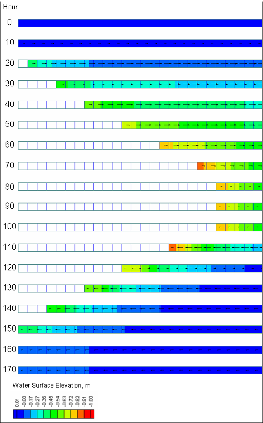
Figure F1. Demonstration of flooding and drying of sloped channel
Test 2: Depression in Square Grid
A source of instability in some flooding and drying algorithms is rewetting of dry cells that surround an area that has formed a pond. A robust flooding algorithm will remain stable with any pattern of wet and dry cells. This test was designed to determine the behavior of the wetting and drying algorithms where ponding takes place.
A square grid consisting of 400 50 ´ 50-m cells was developed in which the central area contained a square ring of shallow cells surrounding deeper cells (Figure F2). Outside the shallow ring, the depth was set to 2 m everywhere. Cells in the shallow ring were specified with depths of 0.3 m, with adjacent interior cells having depths of 0.5 m, and adjacent outer cells having depths of 1.0 m. Four cells in the center of the depression were 1-m deep.
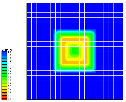
Figure F2. Grid with central depression surrounded by shallow area
The grid was forced with water-surface elevation at six cells located on the left side of the grid, denoted by the red line in Figure F2. A sinusoidal forcing was applied having amplitude of 1 m and period of 12 hr. The depth at which cells are deemed dry was specified as 0.05 m. The model was run for duration of 50 hr, with a ramp of 1 day and time step of 5 s. Plots of water level and circulation are shown in Figures F3 through F10 at hourly intervals starting at hour 42. During hours 43 to 47, the water level was lowered to expose the ring of shallow cells. The dry cells are denoted by white with no current vectors. A pond was formed within the interior of the ring of dry cells.
Water level rises from hours 45 through 49. At hour 46 (Figure F7), cells on the outer portion of the shallow ring (with ambient depths of 1 m) have rewetted. By hour 48 (Figure F9), all previously dry cells have rewetted. During the process of flooding and drying, no instabilities were encountered. Thus, the wetting and drying algorithms in CMS-M2D function properly for the situation of flooding around a ponded area.
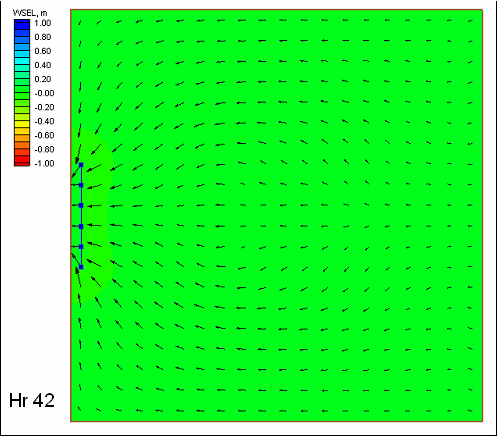
Figure F3. Water level and circulation pattern at hour 42
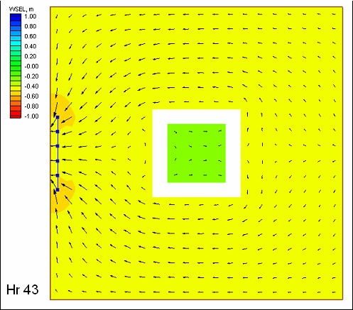
Figure F4. Water level and circulation pattern at hour 43

Figure F5. Water level and circulation pattern at hour 44
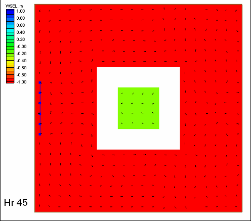
Figure F6. Water level and circulation pattern at hour 45
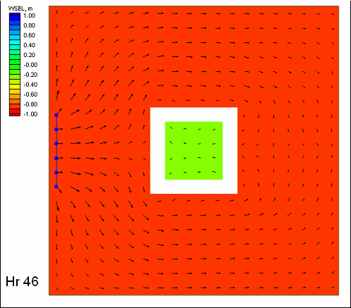
Figure F7. Water level and circulation pattern at hour 46
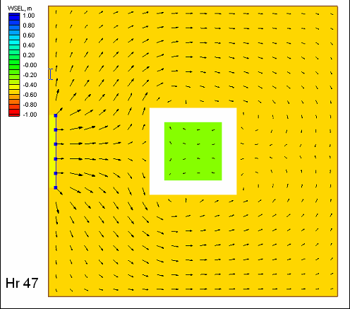
Figure F8. Water level and circulation pattern at hour 47
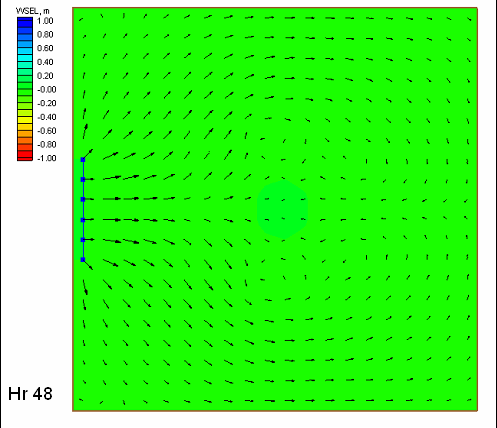
Figure F9. Water level and circulation pattern at hour 48
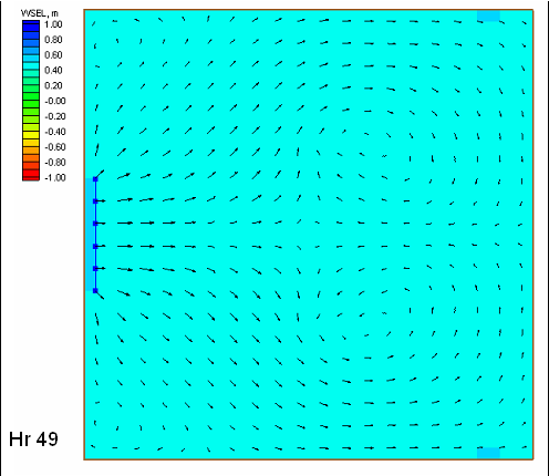
Figure F10. Water level and circulation pattern at hour 49
Appendix G
Wave-Adjusted Boundary Condition Test
This appendix demonstrates the wave-adjusted boundary condition for an idealized beach. In the example, wave forcing is applied to calculate a longshore current. The wave-adjusted boundary condition modifies the water level and velocity on boundaries forced by water-surface elevation to account for the presence of wave forcing. Thus, the prescribed boundary forcing is applied after being adjusted for the presence of waves. This adjustment promotes realistic circulation patterns and wave set up and set down at the boundaries, making values at the lateral boundaries compatible with values calculated within the calculation domain near the boundaries. A simulation without the wave-adjusted boundary condition is also shown, which illustrates the necessity of the modification of water level and velocity at the boundary.
An idealized beach computational grid was developed (Figure G1) having grid spacing of 50 m in each horizontal direction, and depths ranging from 1.13 m at the shoreline to 18.4 m at the seaward boundary. CMS-M2D and STWAVE domains were identical for the idealized beach simulations.
Forcing for the models was specified as:
| a. | STWAVE: Wave height of 2.0 m, period of 10.0 s, and wave angle of 25.0 deg. Spectral spreading parameters werey=3.3 and nn = 4. |
| b. | CMS-M2D: Water-surface elevation set to 0.0 m along lateral and seaward boundaries. |
CMS-M2D was run for 12.5 hr with a 2-s time step and ramp duration of 0.02 day. Results from the simulation without the wave-adjusted boundary condition are described first, followed by those with the wave-adjusted boundary condition.
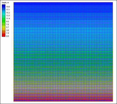
Figure G1. Computational grid for idealized beach
Water-surface elevation and velocity as computed by the standard water-surface elevation forcing boundary condition (boundaries not adjusted for presence of wave forcing) are shown in Figures G2 and G3, respectively. Set up is calculated at the shoreline, but decreases to zero at the lateral boundaries. A longshore current is develops in the nearshore area, but velocities at the lateral boundaries are weaker than inside the calculation domain and display unrealistic patterns. The unrealistic velocity patterns and water-surface elevations at the lateral boundaries owe to the absence of the wave stresses there.
Water-surface elevation and velocity as computed by the wave-adjusted boundary condition are shown in Figures G4 and G5, respectively. Set up is calculated at the shoreline and extends nearly uniformly across the entire grid. An alongshore current is well developed in the nearshore area, both near the lateral boundaries and away from them. Because the boundary conditions were adjusted for the presence of wave forcing, the circulation patterns are realistic. Water can flow onto and off of the grid along the lateral boundaries without incompatibility between the boundary condition and interior hydrodynamic processes.
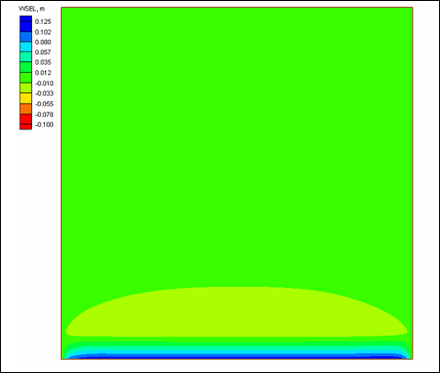
| Figure G2. | Water-surface elevation calculated with standard water surface elevation boundary condition |
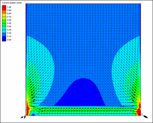
| Figure G3. | Velocity calculated with standard water-surface elevation boundary condition |
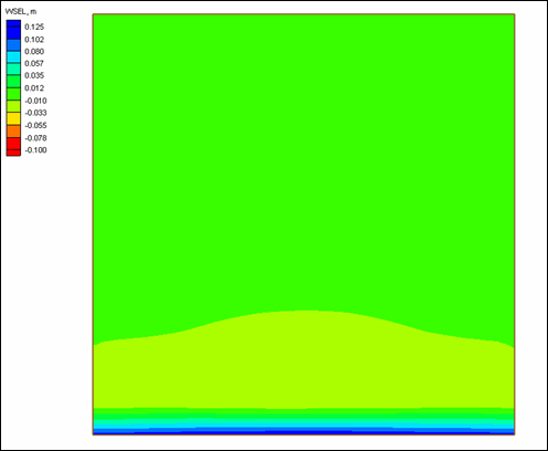
| Figure G4. | Water-surface elevation calculated with wave-adjusted boundary condition |
Figure G5. Velocity calculated with wave-adjusted boundary condition
Appendix H
Surf Zone Verification Tests
To verify CMS-M2D’s response to wave forcing, calculations were compared to laboratory data collected by Visser (1982).[3] Because the laboratory experiments were conducted with monochromatic waves and the bathymetry was uniform alongshore, CMS-M2D was modified to include a 1D monochromatic wave-transformation model. This model applies linear wave theory to compute wave transformation and computes wave height of depth-limited breaking and broken waves by the wave stability relationship of Dally et al. (1985). It also includes representation of the wave roller as described by Dally and Brown (1995) and Dally and Osiecki (1994). Water levels calculated by CMS-M2D are passed to the wave transformation model to allow waves to respond to the set up and set down.
Larson and Kraus (2002) provide succinct descriptions of the wave stability relationship and roller model together with comparisons of calculated and measured longshore current, including comparisons to the Visser (1982) data, with and without the roller model. Their results demonstrate that inclusion of the roller momentum for calculation of the longshore current and wave set up increases accuracy. Without the roller momentum, peak longshore current was calculated to be seaward of the measured peak, whereas including the roller shifted the peak toward the beach and aligned it with the measured peak. This adjustment of the cross-shore distribution of the longshore current modified the set up with an increased set up with the roller as compared to without it.
Calculation of longshore current and set up are conducted for two of the Visser (1982) data sets, Cases 4 and 7. Wave properties for each case are listed in Table H1, and cross-shore profiles and roughness information are listed in Table H2. The major difference between these two cases is the bottom roughness. Case 4 was run on a smooth concrete bottom, whereas bottom roughness elements were introduced for Case 7, with the wave conditions held to be the same as much as possible. By choosing these two tests, performance of CMS-M2D in the surf zone over a great difference in bottom roughness can be demonstrated.
| Table H1 Wave Properties at Offshore End of Basin and Breaker-to-Depth Ratio for Selected Visser (1982) Laboratory Experiments | ||||
| Case | Wave Height, m | Wave Period, s | Wave Angle, deg | Breaker to Depth Ratio |
| 4 | 0.076 | 1.02 | 19.9 | 0.83 |
| 7 | 0.078 | 1.02 | 18.4 | 0.74
|
| Table H2 Cross-Shore Profiles and Roughness Information for Selected Visser (1982) Laboratory Experiments | ||||
| Case | Distance Across Shore, m | Depth, m | Beach Slope1 | Bottom Roughness |
| 4 | -0.472 7.328 8.253 |
-0.040 0.350 0.350 |
0.050 | smooth |
| 7 | -0.472 7.328 9.503 |
-0.040 0.350 0.350 |
0.050 | rough |
| 1 Beach slope calculated for sloping portion of basin.
| ||||
Computational grids were developed for each bathymetric profile, and depths were uniform alongshore. For each grid, the cell spacing parallel to the alongshore direction (Δy) was 0.10 m. Cell spacing parallel to the cross-shore direction (Δx) was 0.01 m from the offshore boundary to approximately 1 m from the shoreline. Resolution was increased nearer to the shore to capture details of the set up calculation. As an example, resolution change for the Case 7 computational grid is shown in Figure H1.
Simulations were conducted with identical parameter settings and time step, with the exception of the Manning roughness coefficient and the breaker-to-depth ratio for which settings were case dependent. The depth at which cells were specified as dry was 0.001 m and the time step was 0.025 s. Breaker-to-depth ratios for each case are provided in Table H1. The Manning roughness coefficient, serving as an adjustment parameter, was set to 0.0125 for Case 4 and to 0.022 for Case 7, after numerical experimentation. Wave calculations proceeded shoreward until a minimum wave height of 0.001 m was reached.
| Figure H1. | Detail of computational grid for Case 7 showing cross-shore variation in cell spacing
|
Comparison of measurements and calculations for wave height, longshore current speed, and set up for Case 4 are shown in Figures H2, H3, and H4, respectively. Calculated wave height compared well with measurements, except for the maximum wave height, which was underestimated by the wave-transformation model. The calculated breakpoint took place directly shoreward and nearly at the measured location.
Calculated longshore current speed well reproduced the distribution determined by the measurements (Figure H3). Peak current speeds compare well, with the calculated peak located directly seaward of the measured peak. Seaward of the breakpoint, calculated weakening of the longshore current closely follows the measured reduction in current.
Set up calculations also compare favorably to the measurements (Figure H4). The slope of the set up is slightly reduced in the calculations as compared to measurements, but the overall result indicates that the model is reproducing the wave-induced set up.
Comparison of calculated and measured wave height and longshore current speed for Case 7 (artificial roughness) are shown in Figures H5 and H6, respectively, and calculated set up is shown in Figure H7 (set up measurements are not available for Case 7). Calculated peak wave height underpredicts the measured peak wave height. However, because measured wave heights before breaking are not available, there is no indication of whether strong nonlinear shoaling took place. Calculated longshore current speed closely matches measurements over the peak and offshore reduction in speed.
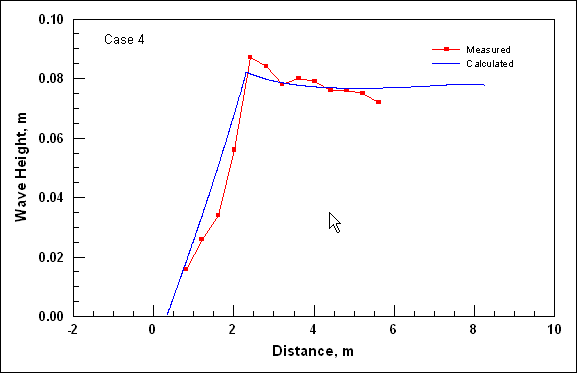
Figure H2. Wave height comparison for Case 4
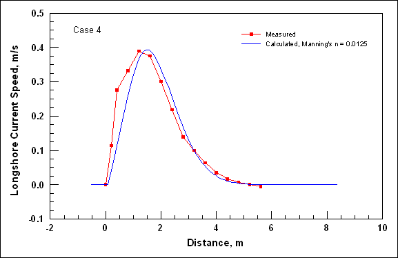
Figure H3. Longshore current comparison for Case 4
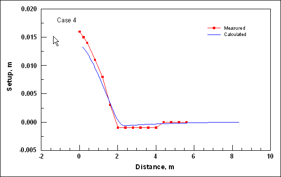
Figure H4. Wave-induced set up comparison for Case 4
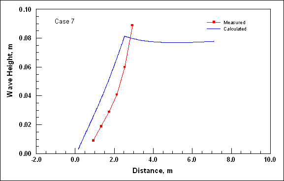
Figure H5. Wave height calculated by roller model for Case 7
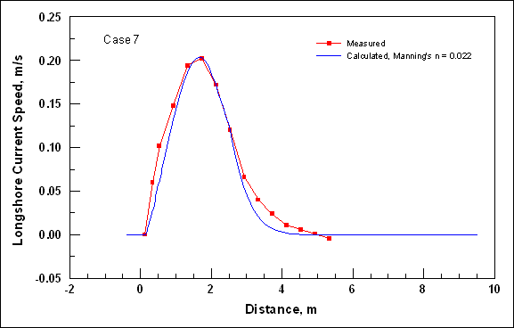
Figure H6. Longshore current calculated by M2D for Case 7
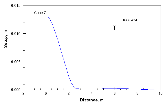
Figure H7. Wave-induced set up calculated by M2D for Case 7
In conclusion, calculations with CMS-M2D well reproduced the qualitative and quantitative features of accurate measurements of the longshore current in the laboratory. This test validates the overall equation solution scheme of the model and contributions of several terms, including the radiation stresses, bottom friction, and mixing.
Appendix I
Hard-Bottom Tests
Functioning of the hard-bottom algorithm within CMS-M2D is demonstrated through two idealized tests that are designed to show calculation properties of the capability. Specifically, demonstrated properties are:
| a. | Hard-bottom cells do not erode below the depth of the non-erodible substrate. |
| b. | Symmetry in depth change calculations for symmetric flow and bathymetry. |
| c. | Hard-bottom cells can accrete and erode sand above the non-erodible substrate. |
| d. | Sand volume is conserved. |
Both tests applied the Watanabe total load sediment transport formulation, and sand size was specified as 0.2 mm.
Test 1: Hard-Bottom Calculations Under Symmetric Conditions
Test 1 was designed to demonstrate that the hard-bottom algorithm does not allow erosion of hard substrate, but does allow accumulation of sand over the non-erodible surface. This example also demonstrates symmetry of the methodology and capability to represent complex configurations of non-erodible cells. The bathymetric configuration (Figure I1) was specified to be a plane horizontal bottom with a pyramid-shaped shoal in the center. The configuration was subject to sediment transport generated by a constant and uniform current in four different simulations where the current originated from each of the four sides of the square. All simulations gave the same symmetrical result relative to the main current direction, so that results from only one direction are provided.
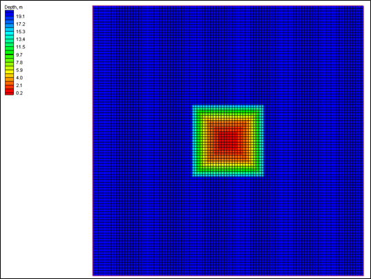
Figure I1. Model bathymetry with cells shown
Figure I2 shows the simulation where the current is directed from the left side. Because of the presence of the pyramidal sediment mound, the current bends around the structure as indicated in the figure. Under the influence of the current, the pyramid erodes.
Figure I3 shows a magnification of the center of the grid. Cells with triangles are specified as having a non-erodible bottom at the initial cell depth (i.e., no sediment cover on the hard-bottom layer). Two sets of runs are compared. In the first set, the hard bottom is not in place, i.e., allowing the cells to erode. In the second set, the hard-bottom cells are in place, limiting erosion to a specified hard-bottom depth. Erosion below the hard-bottom level is allowed in these cells during the first set of runs, but not during the second set.
The result of this comparison is shown in Figure I4, displaying the change in depth (blue denotes erosion, and yellow/red denote accretion) after 7 hr of simulation with no hard-bottom cells present (triangles are retained in the image for reference to previous figure). Cells specified as hard bottom in the following set of simulations erode in the present simulation, indicating that the hydrodynamic conditions cause the bottom to erode below the level of the hard-bottom depth specified in the following simulation. The depth change pattern is symmetric. Figure I5 shows the same situation, but with the hard bottom in place. The calculations show that there is no erosion below the hard-bottom cells. Also, symmetry is preserved.
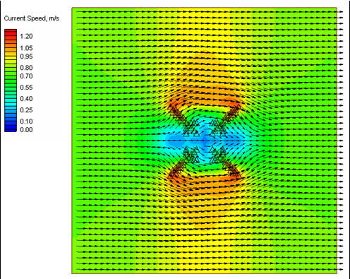
Figure I2. Velocity field over the schematized bottom
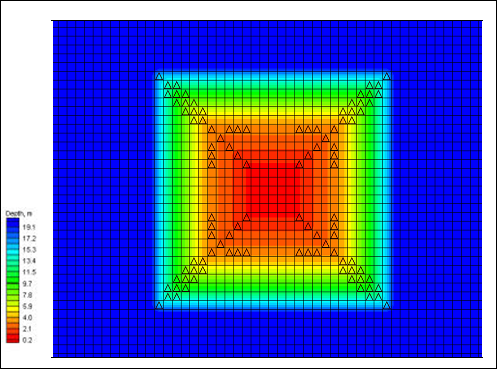
| Figure I3. | Magnification of bathymetry at the center of grid. Cells with triangles are specified as having hard bottom |
Although not shown here, other simulations with the current originating from the other three sides of the square gave the same symmetrical results relative to the main current direction. In all simulations, sand volume was conserved.
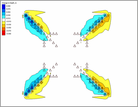
| Figure I4. | Change in depth after 7 hr of simulation without hard-bottom cells (triangles are left in image for reference to previous figure). Blue denotes erosion; yellow/red denote accretion |
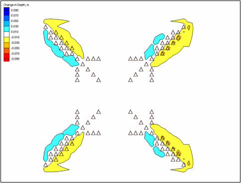
| Figure I5. | Change in depth after 7 hr of simulation with hard-bottom cells. Blue denotes erosion and yellow/red denote accretion |
Test 2: Erosion and Accretion of Sand Over Hard Substrate
A computational grid was developed representing a canal with a shallow region located in its center (Figure I6). Grid depths vary along the x-axis and are uniform along the y-axis. In Figure I6, cells having hard substrates are denoted with triangles. During the simulation, these cells will erode to the hard-bottom surface, then undergo deposition and erosion. The hard- bottom depth was specified to be 0.7 m, and initial grid depths at these cells were 0.5 m, meaning that 0.2 m of sand covered the hard substrate at the beginning of the simulation.

| Figure I6. | Computational grid and bathymetry for demonstration of erosion and deposition of sand over hard substrate. Triangles denote hard-bottom cells |
A 400-hr simulation was conducted in which the current flowed to the right (positive) for 200 hr and then to the left (negative) for 200 hr, establishing conditions for both erosion and deposition at the hard-bottom cells. Time series of current velocity and depth at one hard-bottom cell are shown in Figure I7. During the first 90 hr of the simulation, scour of the sand layer takes place. Once the hard-bottom substrate is reached, scour ceases and the depth remains constant at 0.7 m until current velocities are weak enough for shoaling to start (approximately hour 210). Sand accumulates until the current is strong enough to begin erosion (approximately hour 280), and the erosion continues until the hard substrate is reached again. Thus, the hard-bottom algorithm functions correctly for situations in which sand overlays the hard substrate and erosion takes place to the level of the hard bottom, and for situations in which conditions become depositional at hard-bottom cells.
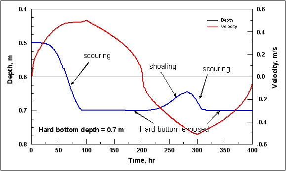
| Figure I7. | Time series of depth of bottom and velocity for demonstration of scour and accumulation of sand over hard substrate |
- ↑ References cited in this appendix are included in the References section at the end of the main text of this report.
- ↑ All references cited in this appendix are included in the References section at the end of the main text.
- ↑ All references cited in this appendix are included in the References section at the end of the main text.

