Spure Dike: Difference between revisions
Created page with " <font size = "4">'''Experiment Setup'''</font> The laboratory flume experiment of Rajaratnam and Nwachukwu (1983) consists of a rectangular 37 x 0.92 m flume with open-c..." |
|||
| (10 intermediate revisions by the same user not shown) | |||
| Line 1: | Line 1: | ||
<big> | |||
__NOTOC__ | |||
==Experiment Setup== | |||
The laboratory flume experiment of Rajaratnam and Nwachukwu (1983) consists of a rectangular 37 x 0.92 m flume with open-channel flow and a thin plate of length 0.1524 m used to simulate a groin-like structure. Here the numerical model is compared to experiment A1 of Rajaratnam and Nwachukwu (1983). For this case, the flow depth and discharge were 0.189 m and 0.0453 m<sup>3</sup>/sec, respectively. | |||
==Model Setup== | |||
The computational grid size is 152 x 36 and has a variable grid resolution of 0.01 to 0.05 m (Figure 1). The mesh was refined manually near the structure, near the walls within the recirculation zone behind the structure. A constant flux was specified at the inflow boundary and a zero water level at the outflow boundary. | |||
[[Image:SpureDikeGrid2.png|thumb|none|1000px|Figure 1. Computational grid for experiment A1 of Rajaratnam and Nwachukwu (1983) .]] | |||
<br style="clear:both" /> | |||
==Results== | |||
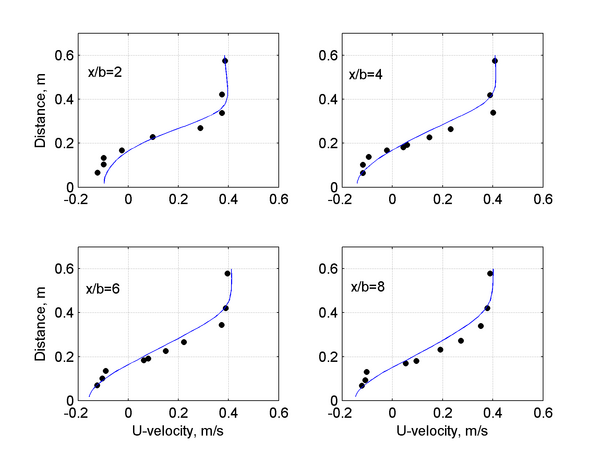
Flow velocities were measured down stream of the flow structure along 4 transects in the transverse direction and at two arbitrary levels or heights y/y0=0.03 and y/y0=0.85. The velocities from y/y0=0.85 are compared to the calculated depth-averaged velocities and are shown in Figure 2. | |||
[[Image:SpureDike_Transects_10k.png|thumb|none|600px|Figure 2. Comparison of measured and computed transect]] | |||
<br style="clear:both" /> | |||
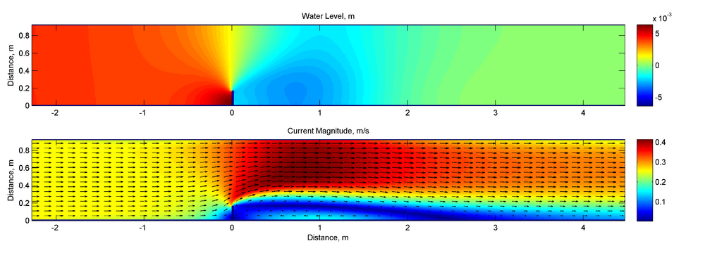
[[Image:SpureDike_Waterlevel_Current_10k.png|thumb|none|1000px|Figure 3.Computed water levels and currents]] | |||
<br style="clear:both" /> | |||
'''Table 1. Goodness of fit statistics for U-velocity, m/s''' | |||
Table 1. Goodness of fit statistics for U-velocity, m/s | |||
{|border="2" cellspacing="0" cellpadding="4" width="79%" | {|border="2" cellspacing="0" cellpadding="4" width="79%" | ||
| | | | ||
|Transect 1 | |'''Transect 1''' || '''Transect 2''' || '''Transect 3''' || '''Transect 4''' | ||
|Transect 2 | |||
|Transect 3 | |||
|Transect 4 | |||
|- | |- | ||
|RMSE | |RMSE || 0.0504 || 0.0690 || 0.0557 || 0.0627 | ||
|0.0504 | |||
|0.0690 | |||
|0.0557 | |||
|0.0627 | |||
|- | |- | ||
|RMAE | |RMAE || 0.0239 || 0.0725 || 0.0884 || 0.1038 | ||
|0.0239 | |||
|0.0725 | |||
|0.0884 | |||
|0.1038 | |||
|- | |- | ||
|R<sup>2</sup> | |R<sup>2</sup> ||0.978 || 0.951 || 0.975 ||0.993 | ||
|0.978 | |||
| 0.951 | |||
| 0.975 | |||
| 0.993 | |||
|} | |} | ||
* For a definition of the goodness of fit statistics see [[Statistics | Goodness of fit statistics]]. | |||
<br style="clear:both" /> | |||
==References== | |||
*Rajaratnam, N. and Nwachukwu, B.A. (1983). "Flow near groin-like structures." ''Journal of Hydraulic Engineering'', 109(3), 463-480. | |||
---- | |||
---- | |||
[[Test_Cases | Test Cases]] | |||
[[CMS#Documentation_Portal | Documentation Portal]] | |||
[[ | |||
Latest revision as of 17:31, 1 June 2011
Experiment Setup
The laboratory flume experiment of Rajaratnam and Nwachukwu (1983) consists of a rectangular 37 x 0.92 m flume with open-channel flow and a thin plate of length 0.1524 m used to simulate a groin-like structure. Here the numerical model is compared to experiment A1 of Rajaratnam and Nwachukwu (1983). For this case, the flow depth and discharge were 0.189 m and 0.0453 m3/sec, respectively.
Model Setup
The computational grid size is 152 x 36 and has a variable grid resolution of 0.01 to 0.05 m (Figure 1). The mesh was refined manually near the structure, near the walls within the recirculation zone behind the structure. A constant flux was specified at the inflow boundary and a zero water level at the outflow boundary.

Results
Flow velocities were measured down stream of the flow structure along 4 transects in the transverse direction and at two arbitrary levels or heights y/y0=0.03 and y/y0=0.85. The velocities from y/y0=0.85 are compared to the calculated depth-averaged velocities and are shown in Figure 2.


Table 1. Goodness of fit statistics for U-velocity, m/s
| Transect 1 | Transect 2 | Transect 3 | Transect 4 | |
| RMSE | 0.0504 | 0.0690 | 0.0557 | 0.0627 |
| RMAE | 0.0239 | 0.0725 | 0.0884 | 0.1038 |
| R2 | 0.978 | 0.951 | 0.975 | 0.993 |
- For a definition of the goodness of fit statistics see Goodness of fit statistics.
References
- Rajaratnam, N. and Nwachukwu, B.A. (1983). "Flow near groin-like structures." Journal of Hydraulic Engineering, 109(3), 463-480.