Wind Setup: Difference between revisions
Jump to navigation
Jump to search
No edit summary |
No edit summary |
||
| (4 intermediate revisions by 2 users not shown) | |||
| Line 4: | Line 4: | ||
== Analytical Solution == | == Analytical Solution == | ||
The analytical solution for wind setup over a constant depth is given by | The analytical solution for wind setup over a constant depth is given by | ||
{{Equation|<math> | |||
\eta = \sqrt{2 \frac{\rho_a C_d W^2}{\rho g} (x + C ) + h^2} - h | |||
</math>|1}} | |||
where <math>\eta</math> is the water surface elevation, <math>\rho</math> is the water density, <math>\rho_a</math> is the air density, <math>g</math> is the gravitational acceleration, <math>W</math> is the wind speed, <math>h</math> is the water depth, and <math>C</math> is a constant of integration. | where <math>\eta</math> is the water surface elevation, <math>\rho</math> is the water density, <math>\rho_a</math> is the air density, <math>g</math> is the gravitational acceleration, <math>W</math> is the wind speed, <math>h</math> is the water depth, and <math>C</math> is a constant of integration. | ||
[[Image: | == Model Setup == | ||
A computational grid with constant water depth of 5 m and irregular boundaries is used in order to test the model performance. The computational grid has 60 columns and 70 rows and a constant resolution of 500 m. | |||
== Results == | |||
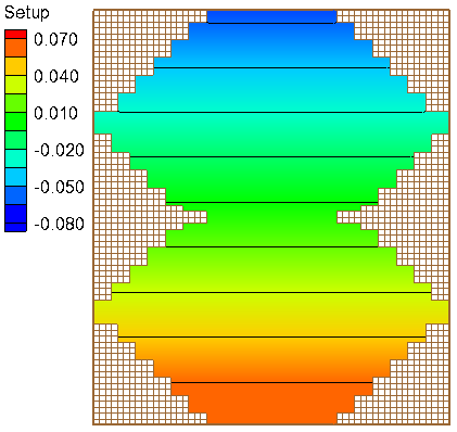
[[Image:Wind_Setup_Dir0_WSE.png|thumb|left|600px| Figure 1. Computed water surface elevation for the irregular domain with constant water depth.]] | |||
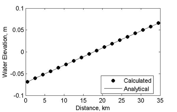
[[Image:Wind_Setup_Dir0_V2.png|thumb|none|600px| Figure 2. Comparison of computed water surface elevation to the analytical solution for an irregular basin with constant depth.]] | |||
<br style="clear:both" /> | <br style="clear:both" /> | ||
Latest revision as of 20:16, 18 April 2013
UNDER CONSTRUCTION
Analytical Solution
The analytical solution for wind setup over a constant depth is given by
| (1) |
where is the water surface elevation, is the water density, is the air density, is the gravitational acceleration, is the wind speed, is the water depth, and is a constant of integration.
Model Setup
A computational grid with constant water depth of 5 m and irregular boundaries is used in order to test the model performance. The computational grid has 60 columns and 70 rows and a constant resolution of 500 m.
Results

