CMS-Flow Multiple-sized Sediment Transport: Difference between revisions
Update CMS Flow Screenshot, Steps V.13.2.12 |
|||
| (63 intermediate revisions by 2 users not shown) | |||
| Line 1: | Line 1: | ||
The CMS multiple-sized sediment transport model is calculated using the multifraction approach, in which the total sediment transport is equal to the sum of the transports of discrete sediment sizes classes. | |||
The input information for multiple-sized sediment transport can be divided into the following groups: | The input information for multiple-sized sediment transport can be divided into the following groups: | ||
| Line 12: | Line 11: | ||
= Grain Size Specification = | = Grain Size Specification = | ||
In the multiple-sized sediment transport model, the continuous grain sizes are divided into discrete bins or size classes. Each size class has a character diameter, and lower and upper limits. Because sediment sizes classes are | In the multiple-sized sediment transport model, the continuous grain sizes are divided into discrete bins or size classes. Each size class has a character diameter, and lower and upper limits. Because sediment sizes classes are transported from one cell to another, the size classes must be constant over the whole domain. In CMS there are two options for specifying the grain size information: | ||
# Characteristic diameters | # Characteristic diameters | ||
# Size class limits | # Size class limits | ||
The characteristic diameters <math> d_k </math> are calculated using the geometric mean of the lower <math> d_{l,k}</math> and upper <math> d_{u,k}</math> bin limits | The characteristic diameters <math> d_k </math> are calculated using the geometric mean of the lower | ||
{{Equation| <math> d_k = \sqrt{d_{l,k} d_{u,k}} </math> | | <math> d_{l,k}</math> and upper <math> d_{u,k}</math> bin limits | ||
{{Equation | <math> | |||
d_k = \sqrt{d_{l,k} d_{u,k}} | |||
</math>| 1}} | |||
The bin width is | |||
The bin width is given by | |||
{{Equation | <math> | |||
\Delta d_k = d_{u,k} - d_{u,k} | |||
</math> | 2}} | |||
The table below describes the CMS-Flow cards related to the grain size class information. | The table below describes the CMS-Flow cards related to the grain size class information. | ||
| Line 41: | Line 47: | ||
'''Recommendations: ''' | '''Recommendations: ''' | ||
* Because each grain size requires the iterative solution of a separate transport formula, it is recommended to not use more 8-9 sediment size classes. For most cases, 3-5 sediment size classes is sufficient. | * Because each grain size requires the iterative solution of a separate transport formula, it is recommended to not use more 8-9 sediment size classes. For most cases, 3-5 sediment size classes is sufficient. | ||
* A good and simple way of estimating the grain size classed based only on the size limits of the distribution is by distributing the diameters logarithmically so that | |||
{{Equation | <math> | |||
d_k = \exp{ \biggl[ \ln{d_1} + \ln{(d_N/d_1)} \frac{k-1}{N-1} } \biggr] | |||
</math> | 3}} | |||
== Matlab Example == | |||
[[Image:Grain_size_distribution.png|thumb|right|500px| Computed grain size distribution.]] | |||
In order to determine the appropriate grain sizes for a simulation it is useful to be able to determine ahead of time the size class fractions using a log-normal distribution for different median grain sizes and sorting. The Matlab example below determines the grain size distribution given the smallest and largest grain sizes, number of sediment sizes, median grain size and geometric standard deviation. The figure shows the computed grain size distribution. | |||
<font size=2> | |||
clear <font color=magenta>all</font>; close <font color=magenta>all</font> | |||
<font color=green>%--- Start Input --- </font> | |||
d1 = 0.234; <font color=green>%mm, smallest grain size </font> | |||
dn = 2; <font color=green>%mm, largest grain size </font> | |||
nsed = 5; <font color=green>%number of grain sizes </font> | |||
d50 = 0.4; <font color=green>%mm, median grain size </font> | |||
sg = 1.5; <font color=green>%mm, geometric standard deviation</font> | |||
<font color=green>%--- End Input --- </font> | |||
<font color=green>%Characteristic diameters </font> | |||
d = exp(log(d1) + log(dn/d1)*((1:nsed)-1.0)/(nsed-1)); | |||
<font color=green>%Limits or bounds</font> | |||
dlim = zeros(1,nsed+1); | |||
dlim(2:nsed)=sqrt(d(2:nsed).*d(1:nsed-1)); | |||
dlim(1)=d(1)*d(1)/dlim(2); | |||
dlim(nsed+1)=d(nsed)*d(nsed)/dlim(nsed); | |||
<font color=green>%Fractions </font> | |||
p = diff(dlim).*lognpdf(d,log(d50),log(sg)); | |||
p = p/sum(p); | |||
<font color=green>%Plotting </font> | |||
figure | |||
hold <font color=magenta>on</font> | |||
<font color=blue>for</font> k=1:nsed | |||
fill([dlim(k) dlim(k+1) dlim(k+1) dlim(k)],... | |||
[0 0 p(k) p(k)]*100,0.5*[1,1,1]) | |||
<font color=blue>end</font> | |||
ylabel(<font color=magenta>'Fraction, %'</font>) | |||
xlabel(<font color=magenta>'Grain size, mm'</font>) | |||
set(gca,<font color=magenta>'box'</font>,<font color=magenta>'On'</font>,<font color=magenta>'TickDir'</font>,<font color=magenta>'out'</font>,... | |||
<font color=magenta>'XMinorTick'</font>,<font color=magenta>'OFF'</font>,<font color=magenta>'YMinorTick'</font>,<font color=magenta>'OFF'</font>) | |||
[d',p'] | |||
<font color=blue>return</font> | |||
</font> | |||
<br style="clear:both" /> | |||
= Fractional Bed Composition = | = Fractional Bed Composition = | ||
| Line 54: | Line 104: | ||
'''Table 2. CMS-Flow card used to specify the option for specifying the bed material composition''' | '''Table 2. CMS-Flow card used to specify the option for specifying the bed material composition''' | ||
{| border="1" | {| border="1" | ||
! Card !! Arguments !! Default | ! Card !! Arguments !! Default !! Range !! Description | ||
|- | |- | ||
| BED_COMPOSITION_INPUT || CHARACTER || D50_SIGMA <nowiki>|</nowiki> D16_D50_D84 <nowiki>|</nowiki> D35_D50_D90 <nowiki>|</nowiki> SIZE_CLASS_FRACTIONS <nowiki>|</nowiki> FRACTIONS_DATASET || Selects the method for specifying the bed material | | BED_COMPOSITION_INPUT || CHARACTER || none || D50_SIGMA <nowiki>|</nowiki> D16_D50_D84 <nowiki>|</nowiki> D35_D50_D90 <nowiki>|</nowiki> SIZE_CLASS_FRACTIONS <nowiki>|</nowiki> FRACTIONS_DATASET || Selects the method for specifying the bed material composition. | ||
|} | |} | ||
| Line 62: | Line 112: | ||
== D50 Dataset and Standard Deviation == | == D50 Dataset and Standard Deviation == | ||
[[ | [[File:CMSFlow Model Parameters SedimentTransportTab V13.2.12.png|thumb|right|400px|Figure 2. ''Sediment'' tab of the ''CMS-Flow Model Control'' window (SMS 13.2.12)]] | ||
This is the simplest and easiest way to specify the bed composition for multiple-sized sediment transport in CMS because it only requires the D50 dataset which is already in the SMS interface and one extra parameter, the geometric standard deviation. | This is the simplest and easiest way to specify the bed composition for multiple-sized sediment transport in CMS because it only requires the D50 dataset which is already in the SMS interface and one extra parameter, the geometric standard deviation. | ||
| Line 72: | Line 122: | ||
<br style="clear:both" /> | <br style="clear:both" /> | ||
The geometric standard deviation <math> \sigma_g </math> can be defined using the method of moments | The geometric standard deviation <math> \sigma_g </math> can be defined using the method of moments | ||
{{Equation| <math | {{Equation | <math> | ||
\sigma_g = \exp{ \sqrt{ \sum p_k(\ln{d_k} - \ln{d_g} )^2 } } | |||
</math> | 4}} | |||
where <math> p_k </math> is the fraction, <math> d_k </math> is the size class diameters in mm, <math> d_g </math> is the geometric mean in mm given by | where <math> p_k </math> is the fraction, <math> d_k </math> is the size class diameters in mm, <math> d_g </math> is the geometric mean in mm given by | ||
{{Equation| <math | {{Equation | <math> | ||
d_g = \exp{ \sum p_k \ln{d_k} } | |||
</math> | 5}} | |||
An alternate approach to | An alternate approach to Equation 5 for obtaining geometric standard deviation is by using the graphical measures (cumulative percentile values) (Folk and Ward, 1957) | ||
{{Equation| <math> \sigma_G = \exp{ \biggl( \frac{\ln{d_{16}} - \ln{d_{84}}}{4} + \frac{\ln{d_5} - \ln{d_{95}}}{6.6} \biggr) } </math> | | {{Equation | <math> | ||
\sigma_g \approx \sigma_G = \exp{ \biggl( \frac{\ln{d_{16}} - \ln{d_{84}}}{4} + \frac{\ln{d_5} - \ln{d_{95}}}{6.6} \biggr)} \approx \biggl( \frac{d_{16}}{d_{84}} \biggr) ^{1/2} | |||
</math> | 6}} | |||
The size class fractions <math> p_k </math> are calculated using log-normal sediment size distribution | The size class fractions <math> p_k </math> are calculated using log-normal sediment size distribution | ||
{{Equation| <math> p_k = \frac{ | {{Equation | <math> | ||
p_k = \frac{\Delta d_k}{ d_k \ln{\sigma_g} \sqrt{2 \pi }} \exp{ \Biggl[ - \frac{1}{2} \biggl( \frac{\ln{d_k} -\ln{d_{50}}}{\ln{\sigma_g}} \biggr)^2 \Biggr] } | |||
</math> | 7}} | |||
<br style="clear:both" /> | <br style="clear:both" /> | ||
'''Table | '''Table 3. Sorting classification based on the geometric standard deviation (Folk and Ward, 1957)''' | ||
{| border="1" | {| border="1" | ||
! Geometric Standard Deviation !! Sorting Classification | ! Geometric Standard Deviation !! Sorting Classification | ||
| Line 124: | Line 182: | ||
# The initial grain size distribution can be approximated by a log-normal distribution | # The initial grain size distribution can be approximated by a log-normal distribution | ||
'''Table | The bed sorting is estimated as | ||
{{Equation | <math> | |||
\sigma_g \approx \biggl( \frac{d_{84}}{d_{16}} \biggr) ^{1/2} | |||
</math> | 8}} | |||
The fractional bed composition is calculated using a log-normal distribution according to Equation 8. | |||
The table below describes the CMS-Flow cards used for specifying the bed material composition using the D16, D50, and D84 datasets. | |||
'''Table 4. CMS-Flow cards related to the D16_D50_D84''' | |||
{| border="1" | {| border="1" | ||
! Card !! Arguments !! Default/Format !! Description | ! Card !! Arguments !! Default/Format !! Description | ||
| Line 130: | Line 198: | ||
| D16_DATASET || CHARACTER CHARACTER || [file name] [dataset path and name] || Specifies the D16 dataset path and file name. | | D16_DATASET || CHARACTER CHARACTER || [file name] [dataset path and name] || Specifies the D16 dataset path and file name. | ||
|- | |- | ||
| D50_DATASET || CHARACTER CHARACTER <nowiki>|</nowiki> CHARACTER || [dataset path and name] <nowiki>|</nowiki> [file name] [dataset path and name ]|| Specifies the D50 dataset path and file name. If the file is not specified than it is assumed to be the model | | D50_DATASET || CHARACTER CHARACTER <nowiki>|</nowiki> CHARACTER || [dataset path and name] <nowiki>|</nowiki> [file name] [dataset path and name ]|| Specifies the D50 dataset path and file name. If the file is not specified than it is assumed to be the model grid file (*_grid.h5). | ||
|- | |- | ||
| D84_DATASET || CHARACTER CHARACTER || [file name] [dataset path and name]|| Specifies the | | D84_DATASET || CHARACTER CHARACTER || [file name] [dataset path and name]|| Specifies the D84dataset path and file name. | ||
|- | |- | ||
| CUSTOM_DATASET || CHARACTER CHARACTER || [file name] [dataset path and name]|| Specifies a custom dataset path and file name. The custom dataset can be used for any additional user defined dataset. The name of the dataset must be equal to the variable name. For example the D16 dataset must be named D16 and cannot be myD16. | | CUSTOM_DATASET || CHARACTER CHARACTER || [file name] [dataset path and name]|| Specifies a custom dataset path and file name. The custom dataset can be used for any additional user defined dataset. The name of the dataset must be equal to the variable name. For example the D16 dataset must be named D16 and cannot be myD16. | ||
| Line 138: | Line 206: | ||
=== Custom Datasets === | === Custom Datasets === | ||
[[File:CMS Flow Custom Datasets Data Calculator V.13.2.12.png|thumb|right|400px|Figure 3. Dataset Calculator showing Custom Datasets for D16 and D84. ]] | |||
The first approach of specifying the D16 and D84 datasets is by using the ''Custom Input Datasets'' section under the ''Input'' tab of the ''CMS-Flow Model Control'' window. The advantage of using this approach is that the user can edit the datasets once they are created without having to map each dataset as the ''Elevation'' dataset. It also avoids having to specify the dataset files and names manually in the *.cmcards file. The steps for creating and specifying the D16 and D84 datasets are outlined below: | The first approach of specifying the D16 and D84 datasets is by using the ''Custom Input Datasets'' section under the ''Input'' tab of the ''CMS-Flow Model Control'' window. The advantage of using this approach is that the user can edit the datasets once they are created without having to map each dataset as the ''Elevation'' dataset. It also avoids having to specify the dataset files and names manually in the *.cmcards file. The steps for creating and specifying the D16 and D84 datasets are outlined below: | ||
# Open '' | # Open ''Data>Data Set Toolbox'' menu and go to the ''Math>Data Calculator'' | ||
# To create the D16 dataset, | # To create the D16 dataset, go to Output dataset name | ||
# Name the dataset D16 for the D16 dataset or D84 for the D84 dataset. The names must be correct for CMS to be able to interpret the dataset. | # Name the dataset D16 for the D16 dataset or D84 for the D84 dataset. The names must be correct for CMS to be able to interpret the dataset. | ||
# | # Go to the Calculator and set the initial values by specifying a spatially constant value. | ||
# Click '' | # Click ''Done'' in the ''Dataset Toolbox'' window | ||
# Repeat steps 2 through 5 for the D84 dataset. | # Repeat steps 2 through 5 for the D84 dataset. | ||
# | # To select the new cells files created, go to the CMS-FLow Model Control>Sediment Transport>Bed Composition to assign the datasets to desired layers | ||
# Save the CMS-Flow project | # Save the CMS-Flow project | ||
<br style="clear:both" /> | |||
Once the datasets are created the SMS project explorer will show a folder with the D16 and D84 datasets. | |||
{| border="0" | {| border="0" | ||
| [[ | |[[File:SMS Explorer Datasets Flow Grid V.13.2.12.png|thumb|300px|Figure 4. SMS project explorer showing Custom Datasets for D16 and D84.]] | ||
|} | |} | ||
<br style="clear:both" /> | <br style="clear:both" /> | ||
After saving the CMS-Flow project the project folder will show a new dataset called ''Flow_Shark_input_datasets.h5''. | |||
[[image:Custom_Datasets_Explorer.png|thumb|left|400px| Figure 5. SMS project explorer showing Custom Datasets for D16 and D84.]] | |||
<br style="clear:both" /> | <br style="clear:both" /> | ||
The data structure of the ''Flow_Shark_input_datasets.h5'' file is shown in the Figure below. | |||
[[image:Input_Datasets_D16_D84.png|thumb|left|400px| Figure 6. Structure of the ''Custom Input Datasets'' file shown in XMDFView. ]] | |||
<br style="clear:both" /> | <br style="clear:both" /> | ||
=== Exported Datasets === | === Exported Datasets === | ||
[[image:Create_D16_Data_Calculator.png|thumb|right|500px| Figure | [[image:Create_D16_Data_Calculator.png|thumb|right|500px| Figure 7. SMS project explorer showing Custom Datasets for D16 and D84. ]] | ||
An alternate approach for specifying datasets is by exporting them into XMDF files and then specifying the file names and paths in the ''Advanced'' cards section of the *.cmcmards file. The advantage of this approach is that is allows more flexibility in specifying project alternatives and also works for SMS versions 10.1 and earlier. | An alternate approach for specifying datasets is by exporting them into XMDF files and then specifying the file names and paths in the ''Advanced'' cards section of the *.cmcmards file. The advantage of this approach is that is allows more flexibility in specifying project alternatives and also works for SMS versions 10.1 and earlier. To export the D16 and D84 datasets | ||
:1. Create and initialize the D16 and D84 datasets | |||
::1.1 Click on the menu ''Data'' | ''Data Calculator'' | |||
::1.2 Enter a constant value under the ''Calculator'' section and make sure the ''Output dataset name'' is either D16 or D84. | |||
<br style="clear:both" /> | |||
:2. If necessary, edit the D16 and D84 datasets. | |||
:: As shown in the figure below, it is not possible to edit the D16 and D84 datasets once they are created. A workaround for this is to set either dataset as the ''Elevation'' dataset, which then allows you to edit the dataset. | |||
[[image:Cannot_Edit_D16.png|thumb|left|400px| Figure 8. It is not possible to edit user defined datasets unless they are the Depth, D50, ManningN, Hardbottom, or a Custom Dataset.]] | |||
<br style="clear:both" /> | |||
:: To set the D16 dataset as the ''Elevation'' dataset: | |||
:: 2.1 Click on ''Data'' | ''Map elevation''. | |||
[[image:Map_D16_to_Elevation.png|thumb|left|400px|Figure 9. Mapping of D16 dataset as the ''Elevation'' dataset.]] | |||
<br style="clear:both" /> | |||
:: 2.2 A window titled ''Select Dataset'' will apear. Select the D16 dataset and click ''Select''. | |||
[[image:Select_D16_Dataset.png|thumb|none|200px|Figure 10. ''Elevation'' dataset selection. ]] | |||
<br style="clear:both" /> | |||
:: The D16 dataset will show with a large ''Z'' on the left indicating that it is mapped as the ''Elevation'' dataset. | |||
[[image:D16_Elevation_Dataset.png|thumb|none|400px| Figure 11. SMS window showing D16 dataset mapped as the ''Elevation'' dataset.]] | |||
<br style="clear:both" /> | |||
:: 2.3 Once you are finished editing the dataset, make sure to remap the appropriate dataset as the ''Elevation'' dataset (usually called ''Depth'' dataset). | |||
:3. Export the D16 and D84 datasets to XMDF file(s). The datasets can be exported to the same or separate file. The important thing is that the correct file name is specified in the Advanced Cards. | |||
[[File:CMS Flow Grid Datasets Export V.13.2.12.png|thumb|left|300px| Figure 12. Exporting the D16 and D84 datasets.]] | |||
<br style="clear:both" /> | <br style="clear:both" /> | ||
== D35, D50, and D90 Datasets == | == D35, D50, and D90 Datasets == | ||
This method is very similar to the previous method. The only difference is that the D35 and D90 datasets are used to estimate the bed sorting instead of the more commonly used D16 and D84 datasets. The reason for including this method is that the D35 and D90 datasets are also required for running the Paticle Tracking Model so it reduces the number of datasets that need to be prepared by the user in cases where both models are being run. | |||
* Assumptions: | * Assumptions: | ||
# The initial bed composition may vary spatially according to the | # The initial bed composition may vary spatially according to the D35, D50, and D90 datasets but is constant with depth | ||
# The initial grain size distribution can be approximated by a log-normal distribution | # The initial grain size distribution can be approximated by a log-normal distribution | ||
The geometric standard deviation is estimated as | |||
\begin{equation} \tag{9} \sigma_g \approx \biggl( \frac{d_{90}}{d_{35}} \biggr) ^{0.61} \end{equation} | |||
The fractional bed composition is then calculated with log-normal distribution according to [[#eq.7|Equation 7]]. | |||
The table below describes the CMS-Flow cards used for specifying the bed material composition using D35, D50, and D90 datasets. | |||
'''Table 5. CMS-Flow cards related to the D35_D50_D90 option for specifying the bed material composition''' | |||
{| border="1" | {| border="1" | ||
! Card !! Arguments !! | ! Card !! Arguments !! Default/Format !! Description | ||
|- | |- | ||
| D35_DATASET || CHARACTER CHARACTER || [file name] [dataset path and name] || Specifies the D35 dataset path and file name. | |||
|- | |- | ||
| | | D50_DATASET || CHARACTER CHARACTER <nowiki>|</nowiki> CHARACTER || [dataset path and name] <nowiki>|</nowiki> [file name] [dataset path and name ]|| Specifies the D50 dataset path and file name. If the file is not specified than it is assumed to be the model grid file (*_grid.h5). | ||
|- | |- | ||
| | | D90_DATASET || CHARACTER CHARACTER || [file name] [dataset path and name]|| Specifies the D84dataset path and file name. | ||
|- | |- | ||
| | | CUSTOM_DATASET || CHARACTER CHARACTER || [file name] [dataset path and name]|| Specifies a custom dataset path and file name. The custom dataset can be used for any additional user defined dataset. The name of the dataset must be equal to the variable name. For example the D35 dataset must be named D35 and cannot be myD35. | ||
|} | |} | ||
| Line 209: | Line 298: | ||
# The initial bed composition is constant at every cell and layer for whole domain | # The initial bed composition is constant at every cell and layer for whole domain | ||
'''Table 6. CMS-Flow cards related to the SIZE_CLASS_FRACTIONS option for specifying the bed material composition''' | |||
{| border="1" | {| border="1" | ||
! Card !! Arguments !! Example !! Description | ! Card !! Arguments !! Example !! Description | ||
| Line 216: | Line 306: | ||
== Fractional Composition Dataset == | == Fractional Composition Dataset == | ||
[[image:XMDFView_Fractions_Dataset.png|thumb|right|400px| Figure 3. XMDFView showing the structure and format of the Fractions dataset]] | |||
The is the most data intensive method for specifying the bed material composition. In the method, the fractional bed composition is specified for each grain size class at every cell and bed layer on the grid. Therefore, the grid is a 200x300 cells with 10 initial bed layers and 5 grain size classes, the input data will be 200x300x10x5 = 3.0e6! | |||
It up to the user to make sure that the fraction dataset sums one for each cell. This method is intended for cases such as laboratory experiments where the horizontal and vertical distribution of the sediments is well known or least needs to be specified precisely. The table below describes the CMS-Flow cards related to the fractional composition dataset method. | |||
<br style="clear:both" /> | |||
'''Table 7. CMS-Flow cards related to the FRACTIONS_DATASET option for specifying the bed material composition''' | |||
{| border="1" | {| border="1" | ||
! Card !! Arguments !! | ! Card !! Arguments !! Format !! Description | ||
|- | |- | ||
| BED_FRACTIONAL_COMPOSITION_DATASET || CHARACTER CHARACTER || [<grid file>] [<grid name>//"Datasets/<Name>"] || Fractional bed composition file. Necessary when setting BED_COMPOSITION_INPUT to | | BED_FRACTIONAL_COMPOSITION_DATASET || CHARACTER CHARACTER || [<grid file>] [<grid name>//"Datasets/<Name>"] || Fractional bed composition file. Necessary when setting BED_COMPOSITION_INPUT to FRACTIONS_DATASET. | ||
|} | |} | ||
<br style="clear:both" /> | |||
= Bed Layer Thickness = | = Bed Layer Thickness = | ||
The initial bed layer thickness needs to be specified by the user. There are three methods for specifying the initial bed layer thickness: | |||
:# CONSTANT – User specified constant for all cells and bed layers. | |||
:# LAYER – User specified bed layer thickness for each bed layer and is applied to all cells on the grid. | |||
:# LAYER_DATASET – User specified dataset for each cell and bed layer (3D dataset). | |||
The CMS-Flow cards related to the bed layer specification are described in the table below. | |||
'''Table 1. CMS-Flow cards related to the general parameters''' | '''Table 1. CMS-Flow cards related to the general parameters''' | ||
{| border="1" | {| border="1" | ||
! Card !! Arguments !! Default/Format !! Range !! Description | ! Card !! Arguments !! Default/Format !! Range !! Description | ||
|- | |- | ||
| BED_LAYER_THICKNESS_INPUT || CHARACTER || | | BED_LAYER_THICKNESS_INPUT || CHARACTER || none || CONSTANT <nowiki>|</nowiki> LAYER_THICKNESS <nowiki>|</nowiki> LAYER_DATASET || Sets the method for specifying the sediment bed layer thickness. | ||
|- | |- | ||
| | | BED_LAYER_THICKNESS_DATASET || CHARACTER CHARACTER || none ||[file] [path] || Specifies the bed layer thickness file and dataset path. | ||
|- | |- | ||
| BED_LAYERS_MAX_NUMBER || INTEGER || || || | | BED_LAYERS_MAX_NUMBER || INTEGER || 8 || >= Input bed layers || Sets the maximum number of bed layers. M | ||
|- | |- | ||
| BED_LAYERS_CONSTANT_THICKNESS || | | BED_LAYERS_CONSTANT_THICKNESS || REAL || none || > minimum layer thickness. || Sets the initial bed layer thickness to a constant in meters for all cells and bed layers. | ||
|- | |- | ||
| | | BED_LAYERS_THICKNESS || INTEGER [REAL, REAL,..., REAL] || [N_lay] [thickness 1] ... [thickness N_lay] || none || Sets the thickness for each layer in meters for all cells. | ||
|- | |- | ||
| | | BED_LAYER_MIN_THICKNESS || REAL || 0.01 || none || Sets the minimum layer thickness. Applicable to all bed layers including the mixing layer (layer 1). | ||
|- | |- | ||
| | | BED_LAYER_MAX_THICKNESS || REAL || 0.5 || none || Sets the MAXIMUMlayer thickness. Applicable to all bed layers including the mixing layer (layer 1). | ||
|} | |} | ||
= Mixing Layer = | = Mixing Layer = | ||
The mixing layer is the first layer from the surface which is allowed to exchange (or mix) sediments with the sediment transport. The mixing layer thickness is calculated based on the median grain size and bed form size. The option is also available to set the mixing layer to a constant. The CMS-Flow cards used for setting the mixing layer thickness to a constant is described in the table below. | |||
'''Table 15. CMS-Flow used for setting a constant mixing layer thickness.''' | |||
{| border="1" | {| border="1" | ||
! Card !! Arguments !! Default | ! Card !! Arguments !! Default !! Range !! Description | ||
|- | |- | ||
| MIXING_LAYER_CONSTANT_THICKNESS || | | MIXING_LAYER_CONSTANT_THICKNESS || REAL || none || greater than minimum thickness || Sets the mixing layer thickness to a constant in meters. | ||
|} | |} | ||
* '''Notes:''' | |||
:# Using a larger mixing layer will slow down the temporal change in bed material composition and enhance model stability. | |||
:# Erosional cases tend to have a smaller mixing layer thicknesses and depositional cases tend to have larger mixing layer thicknesses. | |||
:# The mixing layer thickness should NOT be used as a calibration parameter. | |||
= Hiding and Exposure = | |||
The hiding and exposure is an important parameter for multiple-sized sediment transport. Currently, there are no well established coastal sediment transport formulas for nouniform sediments. The most common approach is to adapt single-size transport formulas by applying correction factors. The most common of these factors is the hiding and exposure correction. The implementation of this factor varies depending on the transport formula and usually involves a coefficient (exponent) which needs to be calibrated. Because all of the transport formula used in CMS were originally developed for uniform sediments, there is still a large uncertainty in the value of the hiding and exposure coefficient. It is expected that the hiding and exposure coefficient will be different for different transport formula especially since the implementation of the hiding and exposure correction may be different for different formula. | |||
Table 15. CMS-Flow card used for setting the hiding and exposure coefficient. | |||
{| border="1" | {| border="1" | ||
! Card !! Arguments !! Default/Format !! Range !! Description | ! Card !! Arguments !! Default/Format !! Range !! Description | ||
|- | |- | ||
| HIDING_EXPOSURE_COEFFICIENT || REAL || | | HIDING_EXPOSURE_COEFFICIENT || REAL || 1.0 || 0.4-1.0 || Sets the hiding and exposure coefficient. | ||
| | |||
|} | |} | ||
= Examples = | = Examples = | ||
Latest revision as of 13:29, 6 December 2022
The CMS multiple-sized sediment transport model is calculated using the multifraction approach, in which the total sediment transport is equal to the sum of the transports of discrete sediment sizes classes.
The input information for multiple-sized sediment transport can be divided into the following groups:
- Grain size classes
- Fractional bed composition
- Bed layer thickness
- Mixing layer
- Hiding and Exposure
Further details on each type of information is provided in the sections below.
Grain Size Specification
In the multiple-sized sediment transport model, the continuous grain sizes are divided into discrete bins or size classes. Each size class has a character diameter, and lower and upper limits. Because sediment sizes classes are transported from one cell to another, the size classes must be constant over the whole domain. In CMS there are two options for specifying the grain size information:
- Characteristic diameters
- Size class limits
The characteristic diameters are calculated using the geometric mean of the lower and upper bin limits
| ( 1) |
The bin width is given by
| ( 2) |
The table below describes the CMS-Flow cards related to the grain size class information.
Table 1. CMS-Flow cards related to the grain size classes
| Card | Arguments | Example | Description |
|---|---|---|---|
| SEDIMENT_SIZE_CLASS_NUMBER | INTEGER | 3 | Specifies the number of grain size classes. |
| MULTIPLE_GRAIN_SIZES | INTEGER [REAL, REAL,..., REAL] | 3 0.1 0.2 0.3 | Specifies the number of grain sizes followed by the grain sizes for each size class in mm. |
| SEDIMENT_SIZE_CLASS_DIAMETERS | INTEGER [REAL, REAL,..., REAL] | 3 0.1 0.2 0.3 | Specifies the number of grain sizes followed by the grain sizes for each size class in mm. Same as MULTIPLE_GRAIN_SIZES. |
| SEDIMENT_SIZE_CLASS_LIMITS | INTEGER [REAL, REAL,..., REAL] | 4 0.07 0.15 0.26 0.34 | Specifies the size classes limits. The first entry is the number of size class limits which is one greater than the number of size classes. |
Notes:
- It is only necessary to specify either the size class characteristic diameters or limits. The other will be calculated internally by the model.
Recommendations:
- Because each grain size requires the iterative solution of a separate transport formula, it is recommended to not use more 8-9 sediment size classes. For most cases, 3-5 sediment size classes is sufficient.
- A good and simple way of estimating the grain size classed based only on the size limits of the distribution is by distributing the diameters logarithmically so that
| ( 3) |
Matlab Example
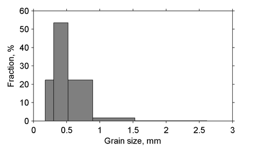
In order to determine the appropriate grain sizes for a simulation it is useful to be able to determine ahead of time the size class fractions using a log-normal distribution for different median grain sizes and sorting. The Matlab example below determines the grain size distribution given the smallest and largest grain sizes, number of sediment sizes, median grain size and geometric standard deviation. The figure shows the computed grain size distribution.
clear all; close all
%--- Start Input ---
d1 = 0.234;  %mm, smallest grain size
dn = 2;      %mm, largest grain size
nsed = 5;    %number of grain sizes
d50 = 0.4;   %mm, median grain size
sg = 1.5;   %mm, geometric standard deviation
%--- End Input ---
%Characteristic diameters
d = exp(log(d1) + log(dn/d1)*((1:nsed)-1.0)/(nsed-1));
%Limits or bounds
dlim = zeros(1,nsed+1);
dlim(2:nsed)=sqrt(d(2:nsed).*d(1:nsed-1));
dlim(1)=d(1)*d(1)/dlim(2);
dlim(nsed+1)=d(nsed)*d(nsed)/dlim(nsed);
%Fractions
p = diff(dlim).*lognpdf(d,log(d50),log(sg));
p = p/sum(p);
%Plotting
figure
hold on
for k=1:nsed
  fill([dlim(k) dlim(k+1) dlim(k+1) dlim(k)],...
    [0 0 p(k) p(k)]*100,0.5*[1,1,1])
end
ylabel('Fraction, %')
xlabel('Grain size, mm')
set(gca,'box','On','TickDir','out',...
  'XMinorTick','OFF','YMinorTick','OFF')
[d',p']
return
Fractional Bed Composition
Since the sediment size classes are constant for the whole domain, the bed composition is specified as the fractional amount of each size class per cell and per bed layer. In CMS V4.0 there are 5 options for specifying the fractional bed composition:
- Two-dimensional horizontal (2DH) D50 dataset plus spatially constant geometric standard deviation (option D50_SIGMA).
- 2DH D16, D50, and D84 datasets (option D16_D50_D84)
- 2DH D35, D50, and D90 datasets (option D35_D50_D90)
- Spatially (horizontally and vertically) constant size class fractions (option SIZE_CLASS_FRACTIONS)
- Fraction of each sediment size class for each cell and bed layer (option FRACTIONS_DATASET)
A description of the CMS-flow card used to select each bed material composition option is described in the Table below.
Table 2. CMS-Flow card used to specify the option for specifying the bed material composition
| Card | Arguments | Default | Range | Description |
|---|---|---|---|---|
| BED_COMPOSITION_INPUT | CHARACTER | none | D50_SIGMA | D16_D50_D84 | D35_D50_D90 | SIZE_CLASS_FRACTIONS | FRACTIONS_DATASET | Selects the method for specifying the bed material composition. |
Further details on each option is provided in the sections below.
D50 Dataset and Standard Deviation
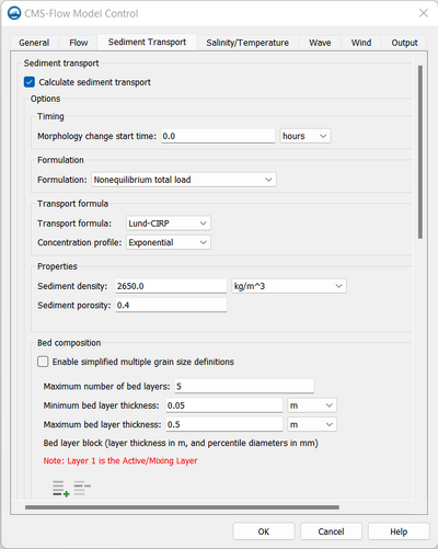
This is the simplest and easiest way to specify the bed composition for multiple-sized sediment transport in CMS because it only requires the D50 dataset which is already in the SMS interface and one extra parameter, the geometric standard deviation.
- Assumptions:
- The initial sediment sorting is constant for the whole domain
- The initial bed composition may vary spatially according to the D50 dataset but is constant with depth
- The initial grain size distribution can be approximated by a log-normal distribution
The geometric standard deviation can be defined using the method of moments
| ( 4) |
where is the fraction, is the size class diameters in mm, is the geometric mean in mm given by
| ( 5) |
An alternate approach to Equation 5 for obtaining geometric standard deviation is by using the graphical measures (cumulative percentile values) (Folk and Ward, 1957)
| ( 6) |
The size class fractions are calculated using log-normal sediment size distribution
| ( 7) |
Table 3. Sorting classification based on the geometric standard deviation (Folk and Ward, 1957)
| Geometric Standard Deviation | Sorting Classification |
|---|---|
| <1.27 | Very well sorted |
| 1.27-1.41 | Well sorted |
| 1.41-1.62 | Moderately well sorted |
| 1.62-2.00 | Moderately sorted |
| 2.00-4.00 | Poorly sorted |
| 4.00-16.00 | Very poorly sorted |
| >16.00 | Extremely poorly sorted |
A description of the CMS-Flow cards related to the D50_SIGMA option for specifying the bed material composition is provided in the table below.
Table 4. CMS-Flow cards related to the D50 dataset and standard deviation
| Card | Arguments | Default/Format | Description |
|---|---|---|---|
| D50_DATASET | CHARACTER CHARACTER | CHARACTER | [file name] [dataset path and name] | Specifies the D50 dataset file followed by the path and name. If the file name is not specified than it is assumed to be the grid file (*_grid.h5). |
| SEDIMENT_STANDARD_DEVIATION | REAL | 1.5 | Specifies the geometric sediment standard deviation for all cells and layers in mm. |
D16, D50, and D84 Datasets
The second approach for specifying the initial bed composition is using 2DH D16, D50, and D84 datasets. Because only the D50 dataset can be specified through the SMS interface, it is necessary to specify the additional datasets either through the Custom Input Datasets are by manually creating the datasets using the Data Calculator and exporting them to XMDF file(s).
- Assumptions:
- The initial bed composition may vary spatially according to the D16, D50, and D84 datasets but is constant with depth
- The initial grain size distribution can be approximated by a log-normal distribution
The bed sorting is estimated as
| ( 8) |
The fractional bed composition is calculated using a log-normal distribution according to Equation 8.
The table below describes the CMS-Flow cards used for specifying the bed material composition using the D16, D50, and D84 datasets.
Table 4. CMS-Flow cards related to the D16_D50_D84
| Card | Arguments | Default/Format | Description |
|---|---|---|---|
| D16_DATASET | CHARACTER CHARACTER | [file name] [dataset path and name] | Specifies the D16 dataset path and file name. |
| D50_DATASET | CHARACTER CHARACTER | CHARACTER | [dataset path and name] | [file name] [dataset path and name ] | Specifies the D50 dataset path and file name. If the file is not specified than it is assumed to be the model grid file (*_grid.h5). |
| D84_DATASET | CHARACTER CHARACTER | [file name] [dataset path and name] | Specifies the D84dataset path and file name. |
| CUSTOM_DATASET | CHARACTER CHARACTER | [file name] [dataset path and name] | Specifies a custom dataset path and file name. The custom dataset can be used for any additional user defined dataset. The name of the dataset must be equal to the variable name. For example the D16 dataset must be named D16 and cannot be myD16. |
Custom Datasets
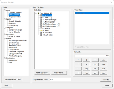
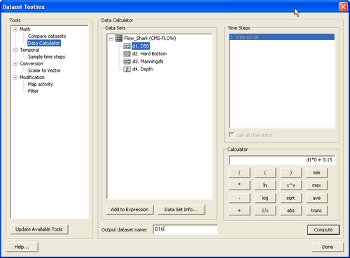
The first approach of specifying the D16 and D84 datasets is by using the Custom Input Datasets section under the Input tab of the CMS-Flow Model Control window. The advantage of using this approach is that the user can edit the datasets once they are created without having to map each dataset as the Elevation dataset. It also avoids having to specify the dataset files and names manually in the *.cmcards file. The steps for creating and specifying the D16 and D84 datasets are outlined below:
- Open Data>Data Set Toolbox menu and go to the Math>Data Calculator
- To create the D16 dataset, go to Output dataset name
- Name the dataset D16 for the D16 dataset or D84 for the D84 dataset. The names must be correct for CMS to be able to interpret the dataset.
- Go to the Calculator and set the initial values by specifying a spatially constant value.
- Click Done in the Dataset Toolbox window
- Repeat steps 2 through 5 for the D84 dataset.
- To select the new cells files created, go to the CMS-FLow Model Control>Sediment Transport>Bed Composition to assign the datasets to desired layers
- Save the CMS-Flow project
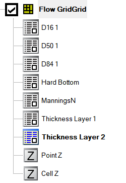
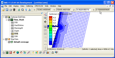
Once the datasets are created the SMS project explorer will show a folder with the D16 and D84 datasets.
 |
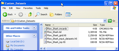
After saving the CMS-Flow project the project folder will show a new dataset called Flow_Shark_input_datasets.h5.
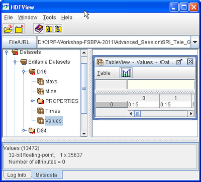
The data structure of the Flow_Shark_input_datasets.h5 file is shown in the Figure below.
Exported Datasets
An alternate approach for specifying datasets is by exporting them into XMDF files and then specifying the file names and paths in the Advanced cards section of the *.cmcmards file. The advantage of this approach is that is allows more flexibility in specifying project alternatives and also works for SMS versions 10.1 and earlier. To export the D16 and D84 datasets
- 1. Create and initialize the D16 and D84 datasets
- 1.1 Click on the menu Data | Data Calculator
- 1.2 Enter a constant value under the Calculator section and make sure the Output dataset name is either D16 or D84.
- 2. If necessary, edit the D16 and D84 datasets.
- As shown in the figure below, it is not possible to edit the D16 and D84 datasets once they are created. A workaround for this is to set either dataset as the Elevation dataset, which then allows you to edit the dataset.
- To set the D16 dataset as the Elevation dataset:
- 2.1 Click on Data | Map elevation.
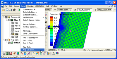
- 2.2 A window titled Select Dataset will apear. Select the D16 dataset and click Select.
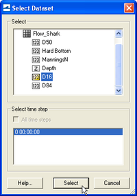
- The D16 dataset will show with a large Z on the left indicating that it is mapped as the Elevation dataset.
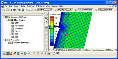
- 2.3 Once you are finished editing the dataset, make sure to remap the appropriate dataset as the Elevation dataset (usually called Depth dataset).
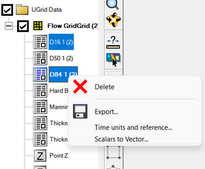
- 3. Export the D16 and D84 datasets to XMDF file(s). The datasets can be exported to the same or separate file. The important thing is that the correct file name is specified in the Advanced Cards.
D35, D50, and D90 Datasets
This method is very similar to the previous method. The only difference is that the D35 and D90 datasets are used to estimate the bed sorting instead of the more commonly used D16 and D84 datasets. The reason for including this method is that the D35 and D90 datasets are also required for running the Paticle Tracking Model so it reduces the number of datasets that need to be prepared by the user in cases where both models are being run.
- Assumptions:
- The initial bed composition may vary spatially according to the D35, D50, and D90 datasets but is constant with depth
- The initial grain size distribution can be approximated by a log-normal distribution
The geometric standard deviation is estimated as \begin{equation} \tag{9} \sigma_g \approx \biggl( \frac{d_{90}}{d_{35}} \biggr) ^{0.61} \end{equation}
The fractional bed composition is then calculated with log-normal distribution according to Equation 7.
The table below describes the CMS-Flow cards used for specifying the bed material composition using D35, D50, and D90 datasets.
Table 5. CMS-Flow cards related to the D35_D50_D90 option for specifying the bed material composition
| Card | Arguments | Default/Format | Description |
|---|---|---|---|
| D35_DATASET | CHARACTER CHARACTER | [file name] [dataset path and name] | Specifies the D35 dataset path and file name. |
| D50_DATASET | CHARACTER CHARACTER | CHARACTER | [dataset path and name] | [file name] [dataset path and name ] | Specifies the D50 dataset path and file name. If the file is not specified than it is assumed to be the model grid file (*_grid.h5). |
| D90_DATASET | CHARACTER CHARACTER | [file name] [dataset path and name] | Specifies the D84dataset path and file name. |
| CUSTOM_DATASET | CHARACTER CHARACTER | [file name] [dataset path and name] | Specifies a custom dataset path and file name. The custom dataset can be used for any additional user defined dataset. The name of the dataset must be equal to the variable name. For example the D35 dataset must be named D35 and cannot be myD35. |
Size Class Fractions
For this case, the fractional bed compositions are specified for each size class for all cells and all bed layers. The fractional bed compositions must sum to 1.0. This option is useful for simulating cases where the bed composition is well known and is constant both in the horizontal and vertical directions.
- Assumption:
- The initial bed composition is constant at every cell and layer for whole domain
Table 6. CMS-Flow cards related to the SIZE_CLASS_FRACTIONS option for specifying the bed material composition
| Card | Arguments | Example | Description |
|---|---|---|---|
| SEDIMENT_SIZE_CLASS_FRACTIONS | INTEGER [REAL, REAL,..., REAL] | 3 0.2 0.5 0.3 | Specifies the fractional composition for each size class and for all cells and bed layers. The first entry is the number of grain size classes. |
Fractional Composition Dataset
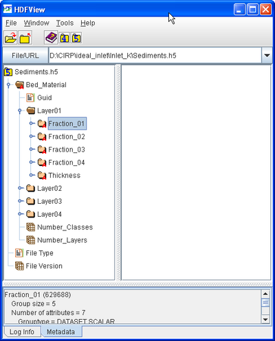
The is the most data intensive method for specifying the bed material composition. In the method, the fractional bed composition is specified for each grain size class at every cell and bed layer on the grid. Therefore, the grid is a 200x300 cells with 10 initial bed layers and 5 grain size classes, the input data will be 200x300x10x5 = 3.0e6!
It up to the user to make sure that the fraction dataset sums one for each cell. This method is intended for cases such as laboratory experiments where the horizontal and vertical distribution of the sediments is well known or least needs to be specified precisely. The table below describes the CMS-Flow cards related to the fractional composition dataset method.
Table 7. CMS-Flow cards related to the FRACTIONS_DATASET option for specifying the bed material composition
| Card | Arguments | Format | Description |
|---|---|---|---|
| BED_FRACTIONAL_COMPOSITION_DATASET | CHARACTER CHARACTER | [<grid file>] [<grid name>//"Datasets/<Name>"] | Fractional bed composition file. Necessary when setting BED_COMPOSITION_INPUT to FRACTIONS_DATASET. |
Bed Layer Thickness
The initial bed layer thickness needs to be specified by the user. There are three methods for specifying the initial bed layer thickness:
- CONSTANT – User specified constant for all cells and bed layers.
- LAYER – User specified bed layer thickness for each bed layer and is applied to all cells on the grid.
- LAYER_DATASET – User specified dataset for each cell and bed layer (3D dataset).
The CMS-Flow cards related to the bed layer specification are described in the table below.
Table 1. CMS-Flow cards related to the general parameters
| Card | Arguments | Default/Format | Range | Description |
|---|---|---|---|---|
| BED_LAYER_THICKNESS_INPUT | CHARACTER | none | CONSTANT | LAYER_THICKNESS | LAYER_DATASET | Sets the method for specifying the sediment bed layer thickness. |
| BED_LAYER_THICKNESS_DATASET | CHARACTER CHARACTER | none | [file] [path] | Specifies the bed layer thickness file and dataset path. |
| BED_LAYERS_MAX_NUMBER | INTEGER | 8 | >= Input bed layers | Sets the maximum number of bed layers. M |
| BED_LAYERS_CONSTANT_THICKNESS | REAL | none | > minimum layer thickness. | Sets the initial bed layer thickness to a constant in meters for all cells and bed layers. |
| BED_LAYERS_THICKNESS | INTEGER [REAL, REAL,..., REAL] | [N_lay] [thickness 1] ... [thickness N_lay] | none | Sets the thickness for each layer in meters for all cells. |
| BED_LAYER_MIN_THICKNESS | REAL | 0.01 | none | Sets the minimum layer thickness. Applicable to all bed layers including the mixing layer (layer 1). |
| BED_LAYER_MAX_THICKNESS | REAL | 0.5 | none | Sets the MAXIMUMlayer thickness. Applicable to all bed layers including the mixing layer (layer 1). |
Mixing Layer
The mixing layer is the first layer from the surface which is allowed to exchange (or mix) sediments with the sediment transport. The mixing layer thickness is calculated based on the median grain size and bed form size. The option is also available to set the mixing layer to a constant. The CMS-Flow cards used for setting the mixing layer thickness to a constant is described in the table below.
Table 15. CMS-Flow used for setting a constant mixing layer thickness.
| Card | Arguments | Default | Range | Description |
|---|---|---|---|---|
| MIXING_LAYER_CONSTANT_THICKNESS | REAL | none | greater than minimum thickness | Sets the mixing layer thickness to a constant in meters. |
- Notes:
- Using a larger mixing layer will slow down the temporal change in bed material composition and enhance model stability.
- Erosional cases tend to have a smaller mixing layer thicknesses and depositional cases tend to have larger mixing layer thicknesses.
- The mixing layer thickness should NOT be used as a calibration parameter.
Hiding and Exposure
The hiding and exposure is an important parameter for multiple-sized sediment transport. Currently, there are no well established coastal sediment transport formulas for nouniform sediments. The most common approach is to adapt single-size transport formulas by applying correction factors. The most common of these factors is the hiding and exposure correction. The implementation of this factor varies depending on the transport formula and usually involves a coefficient (exponent) which needs to be calibrated. Because all of the transport formula used in CMS were originally developed for uniform sediments, there is still a large uncertainty in the value of the hiding and exposure coefficient. It is expected that the hiding and exposure coefficient will be different for different transport formula especially since the implementation of the hiding and exposure correction may be different for different formula.
Table 15. CMS-Flow card used for setting the hiding and exposure coefficient.
| Card | Arguments | Default/Format | Range | Description |
|---|---|---|---|---|
| HIDING_EXPOSURE_COEFFICIENT | REAL | 1.0 | 0.4-1.0 | Sets the hiding and exposure coefficient. |
Examples
- Example 1
SEDIMENT_MAX_ITERATIONS              30
SEDIMENT_STATISTICS                 120.0  720.0
BED_COMPOSITION_INPUT               D50_SIGMA
MULTIPLE_GRAIN_SIZES                6 0.1 0.126 0.16 0.2 0.25 0.31
SEDIMENT_STANDARD_DEVIATION         1.3
BED_LAYER_CONSTANT_THICKNESS        0.5
MIXING_LAYER_CONSTANT_THICKNESS     0.1
MIXING_LAYER_MIN_THICKNESS          0.05
HIDING_EXPOSURE_COEFFICIENT         1.0
SEDMIX_OUT_TIMES_LIST               2
BED_OUT_TIMES_LIST                   2
CALC_MORPH_DURING_RAMP              OFF
- Example 2
SEDIMENT_MAX_ITER                   30
BED_COMPOSITION_INPUT               D50_SIGMA
SEDIMENT_STANDARD_DEVATION          1.5
MULTIPLE_GRAIN_SIZES                5 0.08 0.12 0.17 0.28 0.45
BED_LAYER_CONSTANT_THICKNESS        0.5
MIXING_LAYER_CONSTANT_THICKNESS     0.02
References
- Folk, R.L., and Ward, W.C. (1957). "Brazos River bar: a study in the significance of grain size parameters", Journal of Sedimentary Petrology, 27, 3–26.