Circular Basin: Difference between revisions
No edit summary |
|||
| (One intermediate revision by the same user not shown) | |||
| Line 64: | Line 64: | ||
= Results = | = Results = | ||
== No Coriolis == | == No Coriolis == | ||
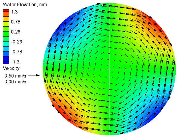
[[Image:CB3_Analytical_No_Coriolis_V4.png|thumb|left| | [[Image:CB3_Analytical_No_Coriolis_V4.png|thumb|left|600px| Figure 1. Analytical current velocities and water levels for the case without Coriolis.]] | ||
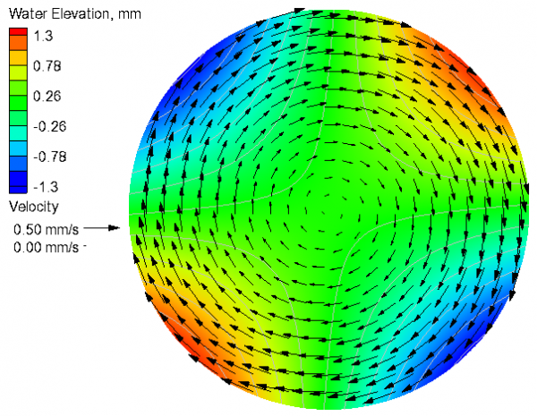
[[Image:CB3_Calculated_No_Coriolis_V5.png|thumb|right| | [[Image:CB3_Calculated_No_Coriolis_V5.png|thumb|right|600px| Figure 2. Calculated current velocities and water levels for the case without Coriolis.]] | ||
<br style="clear:both" /> | <br style="clear:both" /> | ||
Table 2. Goodness of fit statistics for the current velocity and water level | '''Table 2. Goodness of fit statistics for the current velocity and water level.''' | ||
{|border="1" | {|border="1" | ||
|'''Variable''' ||'''NRMSE, %'''||'''NMAE, %'''||'''R^2'''||'''Bias''' | |'''Variable''' ||'''NRMSE, %'''||'''NMAE, %'''||'''R^2'''||'''Bias''' | ||
| Line 83: | Line 83: | ||
== With Coriolis == | == With Coriolis == | ||
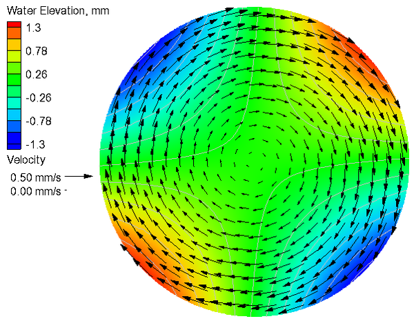
[[Image:CB3_Analytical_Coriolis_V4.png|thumb|left| | [[Image:CB3_Analytical_Coriolis_V4.png|thumb|left|600px| Figure 3. Analytical current velocities and water levels for the case with Coriolis.]] | ||
[[Image:CB3_Calculated_Coriolis_V5.png|thumb|right| | [[Image:CB3_Calculated_Coriolis_V5.png|thumb|right|600px| Figure 4. Calculated current velocities and water levels for the case with Coriolis.]] | ||
<br style="clear:both" /> | <br style="clear:both" /> | ||
Table 3. Goodness of fit statistics for the current velocity and water level | '''Table 3. Goodness of fit statistics for the current velocity and water level.''' | ||
{|border="1" | {|border="1" | ||
|'''Variable''' ||'''RRMSE, %'''||'''RMAE, %'''||'''R^2'''||'''Bias''' | |'''Variable''' ||'''RRMSE, %'''||'''RMAE, %'''||'''R^2'''||'''Bias''' | ||
Latest revision as of 20:07, 18 April 2013
UNDER CONSTRUCTION
Problem
Dupont (2001) presented an analytical solution for a closed circular domain on an f-plane with a linear bottom friction. The governing equations are
| (1) |
| (2) |
| (3) |
where and are the depth-averaged current velocities in the and directions respectively, is the gravitational constant, is the water surface elevation with respect to mean sea level, is a linear bottom friction coefficient, is the radius of the domain, is the water depth, and is a constant equal to the gradient of the wind forcing.
Solution
The analytical solution for water surface elevation solution is given by
| (4) |
The current velocities are independent of the Coriolis parameter and are given by
| (5) |
| (6) |
Setup

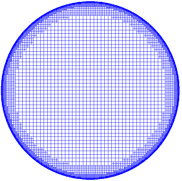
The model is run to steady state from zero current and water level initial conditions with , , and . Table 1 shows the general settings used for CMS-Flow. Figure 1 shows the computational grid with 5 levels of refinement from 2000 m to 125 m.
Table 1. General Settings for Wind-driven flow in a circular basin
| Parameter | Value |
| Time step | 3600 s |
| Simulation Duration | 72 hrs |
| Ramp Period | 24 hrs |
| Initial Water Depth | 100 m |
| Mixing Terms | Off |
| Wall Friction | Off |
| Linear Bottom Friction Coefficient | 0.001 |
Results
No Coriolis


Table 2. Goodness of fit statistics for the current velocity and water level.
| Variable | NRMSE, % | NMAE, % | R^2 | Bias |
| U-Velocity | 2.52 | 0.37 | 0.999 | -8.5e-8 m/s |
| V-Velocity | 2.53 | 0.38 | 0.999 | 7.26e-8 m/s |
| Water Level | 0.03 | 0.02 | 0.999 | -3.5e-7 m |
- For a definition of the goodness of fit statistics see Goodness of fit statistics.
With Coriolis


Table 3. Goodness of fit statistics for the current velocity and water level.
| Variable | RRMSE, % | RMAE, % | R^2 | Bias |
| U-Velocity | 2.53 | 0.37 | 0.999 | -8.5e-8 m/s |
| V-Velocity | 2.56 | 0.37 | 0.999 | 6.5e-8 m/s |
| Water Level | 0.03 | 0.02 | 0.999 | -3.0e-7 m |
References
- Dupont, F., 2001. Comparison of numerical methods for modelling ocean circulation in basins with irregular coasts. Ph.D. thesis, McGill University, Montreal.