User Guide 008: Difference between revisions
No edit summary |
No edit summary |
||
| Line 60: | Line 60: | ||
[[File:fig_2-62.png]] | [[File:fig_2-62.png]] | ||
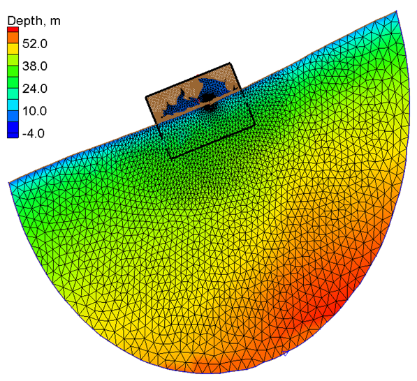
Figure 2 62. Nested CMS-Flow grid within a larger ADCIRC mesh. Note: The ADCIRC mesh was run in geographic coordinates, but was converted to the same horizontal projection as the CMS grid for display. | Figure 2-62. Nested CMS-Flow grid within a larger ADCIRC mesh. Note: The ADCIRC mesh was run in geographic coordinates, but was converted to the same horizontal projection as the CMS grid for display. | ||
=Note<nowiki>:</nowiki>= | =Note<nowiki>:</nowiki>= | ||
| Line 74: | Line 74: | ||
=Tips<nowiki>:</nowiki>= | =Tips<nowiki>:</nowiki>= | ||
:• It is recommended to display both the parent and child computa-tional grids in SMS to check that the horizontal projections are correct and that the grid coverages and bathymetries are | :• It is recommended to display both the parent and child computa-tional grids in SMS to check that the horizontal projections are correct and that the grid coverages and bathymetries are similar. | ||
The input cards used to nest CMS within an ADIRC simulation are pre-sented in the example below. | The input cards used to nest CMS within an ADIRC simulation are pre-sented in the example below. | ||
Revision as of 15:01, 2 May 2015
example 2-44
Single Water Level Time Series
A single water level time-series is one of the most commonly boundary condition types used for coastal modeling.
table 2-55
example 2-45
example 2-46
example 2-47
Multiple Water Level Time Series Boundary
In this boundary condition type, an individual water level time-series is specified for each boundary cell. The SMS 11.1 interface allows the user to extract these time-series from a larger CMS or ADCIRC simulation or to synthesize them from interpolated tidal constituents from a tidal database. Once these time-series are generated, the user can then go into the CMS-Flow Model Control File (*.cmcards file), and use the advanced block structure format to be able to specify additional input options. Specifically, the block structure allows the user to choose a spatial interpolation order, and spatial smoothing along the cellstring. The temporal interpolation is calculated using a piece-wise Lagrangian polynomial of order 1 to 3. The first order polynomial reduces to linear interpolation. The higher order interpolation methods improve the smoothness of the interpolation but can lead to oscillations if the parent simulation is noisy or the solution file output times are very large. This is why the interpolation order is limited to 3. Temporal and spatial smoothing is applied (optional) as central moving averages with a user-specified window width and number of iterations. The spatial smoothing is applied first and then the temporal smoothing to the input boundary water levels. The smoothed water levels are then interpolated to the model time step using the piece-wise Lagrangian interpolation. The boundary water levels may be user-specified in a Time Series Data (TSD) file (*.tsd) or extracted in SMS from a larger simulation or tidal constituent database. Each option is covered in the sections below with examples. The option is also available to output the extracted water levels to a TSD file. The cards used to specify the multiple water level time-series boundary are described in the table below.
table 2-56
Example: SMS-generated Multiple Water Levels
In the example below the SMS interface is used to create a multiple water level time-series boundary and the CMS project files are saved. The CMS-Flow card file is then modified by commenting out the SMS generated card MULTI_HDRIVER_CELLSTRING , and placing the card information in the user-specified boundary block. It is noted that both the cellstring information and the extracted water levels are contained within the same path of the CMS-Flow Model Parameters File (*_mp.h5). This is the reason why both the CELLSTRING and DATASET cards contain the same file name and path. The temporal interpolation order is set to 2, and two iterations of simple moving average filter are applied along the cellstring with a window width of 3.
example 2-48
Example: User-specified Multiple Water Levels
In the example below, a multiple water level boundary condition is speci-fied using all ASCII input files. The cellstring is specified using a BID file, and the boundary water levels using a TSD file.
example 2-49
The TSD file containing the boundary water levels should contain a time series for each boundary cell and covering the whole simulation time period. The format of the TSD file is illustrated in the example below.
example 2-50
Notes:
- • If the number of time steps is set to zero (forth entry in second line of TSD file), CMS will automatically determine the number from the input file. Therefore, the parameter may be considered optional when using as an input for CMS.
Extracted Water Levels from a Parent Simulation
CMS supports automated one-way nesting within parent CMS and ADCIRC models. Additional support for other models is currently in de-velopment. When using this feature, the CMS automatically extracts the boundary condition information from the parent model solution. The user only has to specify the boundary cellstring and the location and name of the parent model simulation files. The user may force the CMS with either water levels or water levels and velocities extracted from the parent simulation.
table 2-57
Note:
•: Simulation results from other models may be used to force CMS by converting them into the ADCIRC format.
table 2-58
Example: Nesting a CMS simulation within an ADCIRC simulation
In the example below, a child CMS simulation is nested within a larger ADCIRC simulation and forced with water surface elevations (WSE). The boundary information begins with user-specified name for the boundary and the cellstring information for the CMS (child) grid. The WSE block contains a WSE offset used in this case to convert between vertical coordinate systems. In addition a small amount of spatial smoothing is applied as a 3 element moving mean along the cellstring. The parent simulation block specifies all of the options of the ADCIRC simulation including the names of the grid, WSE solution files, starting date and time, and horizontal projection. The parent simulation files should include the absolute or relative path if not in the same directory as the CMS (child) simulation. The ADCIRC grid may be specified with the *.14 or *.grd extensions. The default name of the ADCIRC WSE solution file is fort.63 but the fort63.h5 name may also be used. Since the ADCIRC simulation files do not contain information on the starting date or horizontal projection, this information needs to be provided in the model input. Typically, the ADCIRC simulation will be run in a geographic coordinate system.
The simulation domain for both the ADCIRC and nested CMS computa-tional grids is presented in the figure below. In a simulation that the one below, the larger ADCIRC simulation would be forced with tidal constitu-ents while the nested grid is forced with extracted water levels from the ADCIRC simulation.
Figure 2-62. Nested CMS-Flow grid within a larger ADCIRC mesh. Note: The ADCIRC mesh was run in geographic coordinates, but was converted to the same horizontal projection as the CMS grid for display.
Note:
- • ADCIRC is typically run for larger regional grids in a geographic coordinate system. If the horizontal projection is not specified then it is assumed to be NAD83, Geographic with units of degrees.
- • When nesting a CMS simulation within an ADCIRC simulation, it is important that both simulations use the same horizontal datums. Otherwise, the model will not be able to internally convert between the datums.
- • It is important to keep the model forcing for both the parent and child grids consistent. For example if the child grid is forced with winds, then the parent simulation should also be forced with the same winds.
- • Because of differences in resolution, the grid coverages (extents) and bathymetries of the parent and child simulations will never be identical but they should be similar. If they are very different it will lead to boundary problems because the parent model solution will not be consistent with the child model solution.
Tips:
- • It is recommended to display both the parent and child computa-tional grids in SMS to check that the horizontal projections are correct and that the grid coverages and bathymetries are similar.
The input cards used to nest CMS within an ADIRC simulation are pre-sented in the example below.
example 2-51
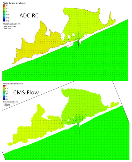
An example comparison of the ADCIRC (parent) and CMS (child) water level solutions is presented in the figure below. The water levels for both simulations are quite close. The differences are mainly due differences in the computational grids.
Figure 2-63. Example snapshots of water levels and current velocities for the ADCIRC (top) and CMS-Flow (bottom) simulations for the same time.
Example: Nesting a CMS simulation within a CMS simulation
If a parent CMS simulation is used, all of the necessary information in-cluding horizontal projection, grid file name, and water level solution file are extracted from the CMS Card File.
example 2-52
Because the CMS-Flow Control (Card) File contains all of the information regarding the horizontal projection, simulation time period, and output files, nothing else needs to be specified except the parent CMS-Flow simulation Card File.
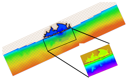
Figure 2-64. Example snapshots of water levels and current velocities for the ADCIRC (top) and CMS-Flow (bottom) simulations for the same time.
Tidal Boundary
In the case of a tidal boundary condition, the external water level is calculated as
| (2-18) |
where
i = subscript indicating a tidal constituent
Ai= mean amplitude [m]
fi= node (nodal) factor [-]
= frequency [deg/hr]
t = elapsed time from midnight of the starting year [hrs]
= equilibrium phase [deg]
= phase lag or epoch [deg]
The external water level is applied equally at all boundary cells unless an inflow
The tidal constituent information is specified using a Tidal Constituent Block and is described in the table below.
table 2-59
The first example for a tidal boundary condition applies two tidal constituents. The constituents are specified by their standard names as listed in Table 2 43, the amplitude in meters, and the phase in degrees. In the example below, the water level block in not included. Since a tidal forcing boundary condition is applied, it implies a water level boundary condition, and all of the default settings are applied to the water level boundary condition.
example 2-53
In second example below, more advanced options are specified. The name is given to the boundary. A water level offset is specified of 0.1 m width respect to the still water level (SWL). The offset is useful for converting from the local vertical datum to the SWL. The direction of the forcing is also specified using the DIRECTION card and produces a phase lag along the tidal boundary condition so that the tidal wave propagates in the direction specified.
example 2-54
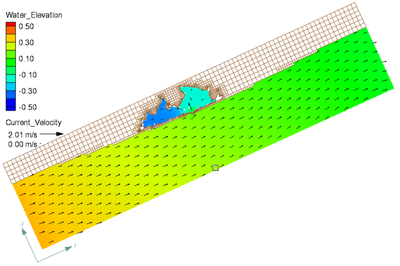
The figure below shows an example of a tidal boundary specified for Shinnecock Inlet NY, with the direction specified parallel to the shoreline for illustration purposes.
Figure 2-65. Example of a tidal boundary condition specified with an incident tidal wave direction parallel to the shore contours (not realistic).
Notes:
- • The water level block may be omitted, since it is understood that a tidal forcing boundary condition applies a water level boundary condition.
Harmonic Boundary
The external water level at a harmonic boundary is calculated as
| Failed to parse (unknown function "\kappi"): {\displaystyle \bar{\eta}_E (t) = \Sigma cos(\omega_i t - \kappi_i)} | (2-19) |
where
i = subscript indicating a harmonic constituent
Ai = mean amplitude [m]
= frequency [deg/hr]
t = elapsed time from the start of the simulation [hrs]
= phase lag or epoch [deg]
The major difference between a tidal and a harmonic boundary condition is that the tidal boundary condition applies corrections to both the ampli-tudes and phases for each constituent which are a function of time while the harmonic boundary does not apply any corrections. Another difference is that in the case of the harmonic boundary, the speed (i.e. frequency) for each constituent must be specified rather than specifying the name of the constituent.
In the first harmonic boundary condition example, only two constituents are specified.
example 2-55
example 2-56
Notes:
- • The water level block may be omitted, since it is understood that a harmonic boundary condition applies a water level boundary condition.


