GenCade Users Guide: Difference between revisions
No edit summary |
No edit summary |
||
| Line 16: | Line 16: | ||
== 1.2 Set the | == 1.2 Set the Current Projection == | ||
GenCade uses a real world coordinate system, so it is necessary to set up the current projection upon opening the SMS. GenCade projects | GenCade uses a real world coordinate system, so it is necessary to set up the current projection upon opening the SMS. GenCade projects may be set up in either U.S. customary units or SI units. The user may select the appropriate projection by clicking ‘’Edit->Projection’’. The steps to set up the projection are shown in Figure 2. This ensures all shorelines, structures, wave gauges, and other important features are mapped correctly. The user may also open aerial photographs to aid in completing the conceptual model. In many cases, the files representing shorelines and other features may be georeferenced correctly without defining the current projection; however, it is a good idea to define the projection before starting a GenCade project. | ||
[[Image: | [[Image:fig2_spec_proj.jpg|400px|thumb|left|Figure 2. Specify projection]] | ||
<br style="clear:both" /> | <br style="clear:both" /> | ||
== 1.3 Reproject | == 1.3 Reproject Current Projection == | ||
In some cases, | In some cases, an aerial photograph may be defined in a different coordinate system than the shorelines. It may also be necessary to develop the conceptual model for the GenCade project in a different coordinate system than the shorelines or aerial photos. In order to change the projection, the user should return to ‘’Edit->Project’’. The window will open, and the user can change the change the projection (Figure 3). | ||
[[Image: | [[Image:fig3_reproject.jpg|400px|thumb|left|Figure 3. Reprojection current projection]] | ||
<br style="clear:both" /> | <br style="clear:both" /> | ||
= 2. Preparing Input Files = | = 2. Preparing Input Files = | ||
== 2.1 Initial | == 2.1 Open and Define Initial Shoreline == | ||
As mentioned previously, an initial shoreline is required to run GenCade. The model type must be defined as ‘’GenCade’’ before opening any file in the SMS. This can be accomplished by selecting ‘’Type->Models->GenCade ‘’ after right clicking on the default coverage under ‘’Map Data’’ in the data tree (panel on left side of screen). If the user has a file with a list of shoreline points that is in the same projection as the project, the file may be opened in the SMS. Before the file is opened in the SMS, it is important to double check the projection of coverage under ‘’Map Data’’. This can be done by right clicking on the coverage and clicking on Projection. If it is necessary to convert to a new projection for the shoreline, right click on the coverage and go to ‘’Reproject’’. A warning will pop up explaining that this is a non-reversible command; select ‘’Yes’’. Then a new window will open allowing the user to define the ‘’Current projection’’ and the ‘’New projection’’. To read the file into the conceptual model correctly, the file must be in *.cst format. The *.cst format requires the x and y coordinates of every point along the shoreline. An example of the format is shown in Figure 4. In order to modify a file with x and y coordinates for a shoreline, add the first three lines shown in Figure 4 which have been carried over from the old GENESIS format. The first number on the third line represents the total number of shoreline points listed in the file. This is the only number in the first three lines that will differ from the file shown in Figure 4. | |||
[[Image: | [[Image:fig4_cst.jpg|400px|thumb|left|Figure 4. Example format of *.cst file]] | ||
<br style="clear:both" /> | <br style="clear:both" /> | ||
[[Image: | There are many different ways to create an initial shoreline for GenCade in the SMS. If the shoreline is represented by points in a shapefile, these can be converted into a scatter set and saved as a text file. Then the text file can be modified to create the proper *.cst format and opened in the SMS. | ||
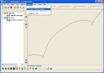
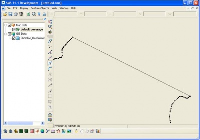
A GenCade initial shoreline can also be created from a polyline shapefile. Once the shapefile is opened in the SMS, it is necessary to click on ‘’Mapping’’ and select ‘’Shapes->Feature Objects’’ (Figure 5). This will create a ‘’Feature Arc’’. After converting the ‘’Map Data’’ to ‘’GenCade’’, the arc may be selected by clicking on the ‘’Select Feature Arc’’ button and by double-clicking. If the shapefile was converted into multiple arcs, it is necessary to connect these segments to create one arc (Figure 6). Click on the ‘’Create Feature Arc’’ button and draw an arc connecting the existing arcs. Click on the ‘’Select Feature Point’’ button and select all of the nodes between the existing and the new arcs. To convert the nodes to vertices, go to ‘’Feature Objects’’ and select ‘’Vertices<->Nodes’’. Once all of the nodes have been converted to vertices, the shoreline is in the proper format for GenCade. When developing a shoreline in GenCade from a polyline shapefile, it is not necessary to create a *.cst file. | |||
[[Image:fig5_convert.jpg|400px|thumb|left|Figure 5. Convert shapefile to feature objects]] | |||
<br style="clear:both" /> | |||
[[Image:fig6_connect.jpg|400px|thumb|left|Figure 6. Connect segments to create one feature arc]] | |||
<br style="clear:both" /> | <br style="clear:both" /> | ||
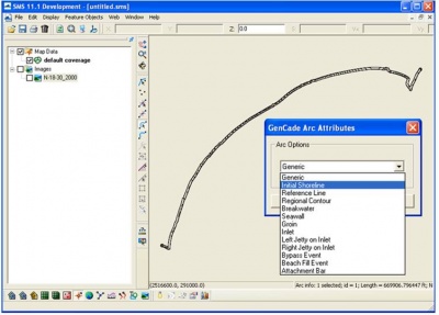
Regardless of whether or not the initial shoreline is opened as a *.cst file, the initial shoreline must be defined. To define the initial shoreline, ‘’GenCade’’ must be selected as the model type for the coverage. The feature arc representing the shoreline should be double-clicked (or right-click and select Attributes) after clicking on the ‘’Select Feature’’ Arc button. The ‘’GenCade Arc Attributes’’ window will open. The ‘’Initial Shoreline’’ option should be selected under ‘’Arc Options’’. These steps are shown in Figure 7. | |||
[[Image: | [[Image:fig7_shoreline.jpg|400px|thumb|left|Figure 7. Define arc as initial shoreline]] | ||
<br style="clear:both" /> | <br style="clear:both" /> | ||
== 2.2 Regional | == 2.2 Open and Define Regional Contour or Additional Shorelines == | ||
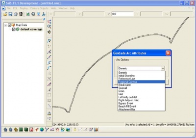
In some cases, | In some cases, a regional contour or additional shorelines may need to be added to the conceptual model. In order to define a second feature arc, it is necessary to right-click on ‘’Map Data’’ and select a ‘’New Coverage’’. This new coverage must also be defined as ‘’GenCade’’. The user can rename the new coverage, so that it can easily be identified. It is very important to open the new arc in a new coverage. If the arc is opened in the same coverage as the initial shoreline, the two arcs will most likely overlap, and the arcs will be split into many arcs. Once the regional contour is opened in the interface, define the arc as ‘’Regional Contour’’ in the ‘’GenCade Arc Attributes’’ window (Figure 8). A shoreline representing the final shoreline or an additional shoreline may be defined as a ‘’Reference Line’’. | ||
[[Image: | [[Image:fig8_rc.jpg|400px|thumb|left|Figure 8. Define arc as regional contour]] | ||
<br style="clear:both" /> | <br style="clear:both" /> | ||
[[Image: | == 2.3 Merge Coverages == | ||
After the initial shoreline and regional contour have been loaded and defined in the SMS interface, it is necessary to merge the two lines in a single coverage. All structures, inlets, wave gages, and other features will be created in this single coverage. Highlight both the default coverage (initial shoreline) and the new coverage (regional contour). This can be done by hitting ctrl on the keyboard and clicking on both coverages. After right-clicking, select ‘’Merge Coverages’’. A window will open asking if the user would like to delete the coverages used to make the merged coverage. If no is selected, the initial shoreline and regional contour coverages will remain in the interface. It is a good idea to keep these coverages in the interface. If a problem occurs with the merged coverage, the initial shoreline and regional contour may be merged again. Figure 9 shows how coverages are merged while Figure 10 illustrates the initial shoreline and regional contour in the merged coverage. | |||
[[Image:fig9_merge.jpg|400px|thumb|left|Figure 9. Merge initial shoreline and regional contour in a single coverage]] | |||
<br style="clear:both" /> | <br style="clear:both" /> | ||
[[Image:fig10_merge.jpg|400px|thumb|left|Figure 10. Arcs for initial shoreline and regional contour defined after merging into a single coverage]] | |||
[[Image: | |||
<br style="clear:both" /> | <br style="clear:both" /> | ||
= 3. Grid Setup = | = 3. Grid Setup = | ||
== 3.1 | == 3.1 Create Inlets, Shoals, Dredging Events, and Jetties == | ||
The inlet name, inlet shoal volumes, dredging events, and bypassing coefficients may be defined when an inlet is created. To do this, select the ‘’Create Feature Arc’’ button and draw a line from one side of the inlet to the other. When creating inlets and other features, a high quality aerial photo is very helpful. After the inlet is created, click on the ‘’Select Feature Arc’’ button and double-click on the arc representing the inlet. This can also be accomplished by a single click, followed by a right click. The ‘’GenCade Arc Attributes’’ window will open. Select ‘’Inlet’’ and click on ‘’Attributes’’. The ‘’Inlet Reservoir Model’’ window will open. The inlet can be named, shoal volume can be defined, and dredging events can be added. The initial and equilibrium shoal volumes for the ebb, flood, left bypass, left attachment, right bypass, and right attachment can be defined after clicking on the ‘’Volume’’ button. Similarly, after clicking on ‘’Dredging’’, the ‘’Dredging Events’’ window will open and the user can specify the beginning and ending date, the volume, and the shoal to be mined for each dredging event. The user also has the option to modify the left and right bypassing coefficients when jetties are present. Both the left and right bypassing coefficients have a default value of 1. Inlets that do not have jetties will not have a bypassing coefficient. After the inlet information is specified, the arc representing the inlet will turn blue. All of the steps create an inlet and add shoal volumes and dredging events are shown in Figure 11. | |||
[[Image: | [[Image:fig11_inlets.jpg|400px|thumb|left|Figure 11. Create and define an inlet, shoal volumes, and dredging events]] | ||
<br style="clear:both" /> | <br style="clear:both" /> | ||
A jetty can be created at the inlet after selecting the ‘’Create Feature Arc’’ button. The arc representing the jetty should not intersect with the arc representing the inlet, regional contour, or initial shoreline. If this occurs, either the arc representing the jetty or the regional contour or initial shoreline will be split into two separate arcs. To remedy the problem of splitting arcs; the user should delete the arc representing the jetty, convert the newly created node to a vertex, and redefine the formerly split arc. After drawing the jetty, the user should click on the ‘’Select Feature Arc’’ and double-click on the line representing the jetty. When the ‘’GenCade Arc Attributes’’ window opens, the ‘’Left Jetty on Inlet’’ or ‘’Right Jetty on Inlet’’ should be selected. The left jetty is to the left of a person standing on land looking at the ocean. After ‘’Attributes’’ is selected, a new window will open where the ‘’Permeability’’ can be specified, ‘’Diffracting’’ can be checked or unchecked, and a seaward depth can be added. The default value for ‘’Permeability’’ is 0. Although ‘’Diffracting’’ is unchecked as a default option, the user should check this box in most cases. The line representing a jetty will also turn blue once all of required jetty information is provided. Figure 12 shows how to create a jetty. | |||
To | |||
[[Image: | [[Image:fig12_jetty.jpg|400px|thumb|left|Figure 12. Create and define a jetty]] | ||
<br style="clear:both" /> | <br style="clear:both" /> | ||
[[Image: | Once the grid is converted to GenCade, the bypassing bars associated with an inlet are defaulted to the one cell immediately adjacent to either side of the inlet. However, the bar size and location may be defined in the conceptual model. After the bar is created, it is necessary to double-click on the arc. Once the ‘’GenCade Arc Attributes’’ window is open, the bar can be defined as an ‘’Attachment Bar’’ (Figure 13). The attachment bar is also represented by a blue line. | ||
[[Image:fig13_attach.jpg|400px|thumb|left|Figure 13. Create and define an attachment bar]] | |||
<br style="clear:both" /> | <br style="clear:both" /> | ||
== 3.2 Seawalls == | |||
To draw a seawall, first the ‘’Create Feature Arc’’ button should be selected. The seawall must be drawn landward of the shoreline. If the user attempts to draw the seawall directly on top of the initial shoreline, an error will occur. The seawall drawn by the user should resemble the shape of the real seawall as closely as possible. If the user is not meticulous in drawing the seawall, the shape of the seawall in the GenCade model may not resemble the actual seawall. Additionally, since cell numbers are used in the GenCade model, the seawall shape may look different after converting from the conceptual model. After the seawall is drawn, the user should click on the Select Feature Arc button and click on the seawall. The ‘’GenCade Arc Attributes’’ window will open. ‘’Seawall’’ should be selected in ‘’Arc Options’’. The seawall will turn blue. When the model is converted to a 1D grid, an error message referring to the seawall may pop up. This message should be ignored; GenCade will modify the cells defined for the seawall. The user should review the seawall in the GenCade model. If the seawall does not resemble the actual seawall, the cell numbers and distances from the grid should be revised. A smaller cell size near the seawall may also be helpful. The process to create a seawall is shown in Figure 14. | |||
[[Image: | [[Image:fig14_seawall.jpg|400px|thumb|left|Figure 14. Create and define a seawall]] | ||
<br style="clear:both" /> | <br style="clear:both" /> | ||
== 3.3 Beach | == 3.3 Beach Fills == | ||
Beach fills can be | Beach fills can be created in the same way as inlets and seawalls. One should select the ‘’Create Feature Arc’’ button to draw the beach fill. Beach fills should be drawn slightly offshore. If there are many beach fills in one location during the simulation, draw the beach fills carefully so they do not connect or intersect. After each beach fill is drawn, click on the ‘’Select Feature Arc’’ and double-click on the line representing the beach fill. Select the ‘’Beach Fill Event’’ after the ‘’GenCade Arc Attributes’’ window opens. For each beach fill, add the ‘’Begin Date’’ and ‘’End Date’’ and the ‘’Added Berm Width’’. After selecting ‘’OK’’ in the ‘’GenCade Arc Attributes’’ window, the line representing the beach fill will turn green. Figure 15 demonstrates the steps to create and define beach fill events. | ||
[[Image: | [[Image:fig15_beach_fill.jpg|400px|thumb|left|Figure 15. Create and define a beach fill]] | ||
<br style="clear:both" /> | <br style="clear:both" /> | ||
== 3.4 | == 3.4 Detached Breakwaters == | ||
A detached breakwater is created by selecting the ‘’Create Feature Arc’’ button and drawing the arc representing the detached breakwater. The user should click on the ‘’Select Feature Arc’’ button and double-click on the detached breakwater. The ‘’GenCade Arc Attributes’’ window will open. Scroll down to ‘’Breakwater’’ and click on ‘’Attributes’’. The depth at each end of the detached breakwater can be entered in the ‘’Detached Breakwater’’ window. There is a pull-down window for wave transmission which includes constant transmission and three equations for time-dependent wave transmission: Ahrens, Seabrook and Hall, and d'Angremond. | |||
[[Image: | === 3.4.1 Constant Transmission === | ||
Under the ‘’Transmission’’ bar, select ‘’Constant’’. The last column in the detached breakwaters window is ‘’Coeff/Perm/Atts’’. For constant transmission, this represents the permeability of the detached breakwater. Once all necessary information is entered, click ‘’OK’’. The detached breakwater will turn orange. A detached breakwater with constant transmission is shown in Figure 16. | |||
[[Image:fig16_breakwater.jpg|400px|thumb|left|Figure 16. Create and define a breakwater with constant transmission]] | |||
<br style="clear:both" /> | <br style="clear:both" /> | ||
== 3. | === 3.4.2 Time-dependent Wave Transmission === | ||
==== 3.4.2.1 Ahrens ==== | |||
After selecting Ahrens under ‘’Transmission’’ in the ‘’Detached Breakwater’’ window, the final column (‘’Coeff/Perm/Atts’’) can be selected. Clicking this box will open the ‘’Breakwater Attributes’’ window. For Ahrens, the required values include freeboard to MSL, width, seaward side slope, shoreward side slope, and the D50 of the armor stone (Figure 17). Click ‘’OK’’, and the detached breakwater should turn orange. | |||
==== 3.4.2.2 d'Angremond ==== | |||
Another equation that can be used for time-dependent wave transmission is d'Angremond. Similarly to the option for ‘’Ahrens’’, click on the final column of the ‘’Detached Breakwaters’’ window which should now say ‘’Atts’’. For d'Angremond, the freeboard to MSL, width, seaward side slope, shoreward side slope, and permeability are required (Figure 18). | |||
==== 3.4.2.3 Seabrook and Hall ==== | |||
Seabrook and Hall can also be used for time-dependent wave transmission. After selecting Seabrook and Hall in the ‘’Detached Breakwaters’’ window, click on ‘’Atts’’ in the final column. The ‘’Breakwater Attributes’’ window will open, and the freeboard to MSL, width, seaward side slope, shoreward side slope, and D50 of the armor stone can be entered (Figure 19). | |||
[[Image:fig17_ahrens.jpg|400px|thumb|left|Figure 17. Define breakwater using Ahren’s method for transmission]] | |||
<br style="clear:both" /> | |||
[[Image:fig18_dangremond.jpg|400px|thumb|left|Figure 18. Define breakwater using d’Angremond method for transmission]] | |||
<br style="clear:both" /> | |||
[[Image: | [[Image:fig19_seabrook_hall.jpg|400px|thumb|left|Figure 19. Define breakwater using Seabrook and Hall method for transmission]] | ||
<br style="clear:both" /> | <br style="clear:both" /> | ||
== 3.5 Groins == | |||
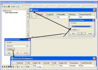
Once the location for a groin is chosen, select the ‘’Create Feature Arc’’ button. In many cases, the arc representing the groin will cross the regional contour and initial shoreline. Do not draw either end of the groin near the regional contour or initial shoreline. When this occurs, the node from the groin will connect to the initial shoreline or regional contour. This will divide the regional contour or initial shoreline into two separate arcs, where only one of the arcs will still be defined as the regional contour or initial shoreline. To remedy this, delete the arc that was created to represent the groin. Highlight the node that divides the initial shoreline into two segments. Under Feature ‘’Objects’’, select ‘’Vertices<->Nodes’’. The node will become a vertex, and the initial shoreline will once again be a single arc. After drawing the feature arc for the groin, click on the ‘’Select Feature Arc’’ button. The ‘’GenCade Arc Attributes’’ window will open. Select ‘’Groin’’ in the ‘’Arc Options’’ menu and click on ‘’Attributes’’. The window for groins is very similar to the window for jetties. The window for groins includes the ‘’Permeability’’ and ‘’Seaward Depth’’ (in the user specified units). The user may also define the groin as ‘’Diffracting’’ or ‘’Non-diffracting’’. When the ‘’Diffracting’’ option is checked, a ‘’Seaward Depth’’ must be specified. Figure 20 illustrates the various windows associated with creating a groin. | |||
[[Image: | [[Image:fig20_groin.jpg|400px|thumb|left|Figure 20. Define and create a groin]] | ||
<br style="clear:both" /> | <br style="clear:both" /> | ||
== 3.6 T-Groins == | |||
While a T-groin is not an arc attribute that can be created and defined in GenCade, a detached breakwater and a groin can be combined to form a T-groin. If a T-groin is required, the user should first create a detached breakwater and fill in all of the information necessary for a detached breakwater in the ‘’GenCade Arc Attributes’’ window. Then the user should create a groin that attaches to the detached breakwater. Once the conceptual model is converted to a 1D grid, it is necessary to double-check the T-groin to ensure that the shape has been retained. It is possible that the groin or detached breakwater has moved to an adjacent cell number and no longer retains the shape the user defined. The user may modify the cells for the detached breakwater or groin in the GenCade model under ‘’Edit Breakwaters’’ or ‘’Edit Groins’’ in the ‘’GenCade’’ menu. An example of a T-groin is shown in Figure 21. | |||
[[Image: | [[Image:fig21_tgroin.jpg|400px|thumb|left|Figure 21. Create a T-groin]] | ||
<br style="clear:both" /> | <br style="clear:both" /> | ||
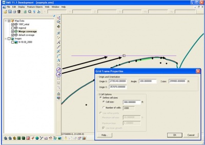
== 3.7 Orientation, Cell Size, and Variable Grid Resolution == | |||
After defining the shorelines and any necessary structures, the grid should be set up. To manually draw the grid frame, click on the ‘’Create 1-D Grid Frame’’. The GenCade grid frame is purple and has an arrow at one end. If a person followed the grid from the end to the arrow, the water should always be to the left and the land should always be to the right. For example, if the GenCade grid was oriented from north to south, the water would be to the east (left) and the land would be to the west (right). The grid can be modified by clicking the ‘’Select 1-D Grid Frame’’ and double-clicking on the square in the center of the purple grid line. Alternately, the grid options can be changed by selecting the grid frame and right-clicking Properties. The ‘’Grid Frame Properties’’ window will open, and the ‘’Origin X’’, ‘’Origin Y’’, ‘’Angle’’, and ‘’I size’’ can be modified. The ‘’I size’’ is the length of the grid. ‘’Angle’’ refers to the sign convention in the conceptual model which is degrees counterclockwise from the x axis. This is different from the GenCade model convention (degrees clockwise from north). Therefore, once the map is converted to a 1D grid, the ‘’Azimuth’’ for the grid will be a different value. The cell size can be constant or variable. If the user chooses to change the cell size under ‘’Define cell sizes’’, the number of cells will change accordingly. The grid frame set up is shown in Figure 22. | |||
[[Image: | [[Image:fig22_grid_frame.jpg|400px|thumb|left|Figure 22. Create and define the grid frame]] | ||
<br style="clear:both" /> | <br style="clear:both" /> | ||
A constant grid resolution is reasonable for most projects. However, there are some large scale projects that would benefit from variable grid resolution. Variable grid resolution can give more detail at specific locations of interest while having coarser resolution in other areas of the grid. By utilizing variable grid resolution, the simulation will run much more quickly than a grid with a constant, finer resolution. When the map is converted to a 1D grid, one of the options under ‘’I Cell Options’’ is ‘’Use refine points’’. This option refers to variable grid resolution. | |||
First, it is necessary to determine which part of the grid needs a finer resolution. There are two ways to set up finer grid resolution. The user can decide to use one point or two points. For both of these options, click the ‘’Create Feature Point’’ button. If only one feature point is created, put the point at the location of interest. Click on the ‘’Select Feature Point’’ button and double-click on the point. The ‘’Refine Point’’ window will open (Figure 23). Check the ‘’Refine grid in I direction’’ and specify a base cell size. The base cell size is the size of the cells nearest to the refine point. This will be the smallest cell size in this location of the grid. Once the refine point is specified, right click on the coverage under ‘’Map Data’’ and convert ‘’Map->1D Grid’’. The ‘’Map->1D Grid’’ window will open (Figure 24). Under I Cell Options, click the button to specify the ‘’Use refine points’’ option. Type the maximum cell size and the maximum bias. The maximum cell size represents the largest cell size in the grid. Moving out from the one refine point, the cells will grow in size until a cell reaches the maximum cell size. The remaining cells in the grid will also be the maximum cell size. The maximum bias represents the amount each adjacent cell grows. For example, the default value is 1.10. This means each cell will grow 10%, so in a case with a base cell size of 10, the adjacent cells will have a size of 11. The cells will continue growing at this rate until a cell reaches the maximum cell size. In a case with only one refine point, do not select the ‘’Use inner growth’’ option. | |||
[[Image:fig23_variable.jpg|400px|thumb|left|Figure 23. Refine the grid for variable resolution]] | |||
<br style="clear:both" /> | |||
[[Image: | [[Image:fig24_refine_pts.jpg|400px|thumb|left|Figure 24. Convert to GenCade grid using refine points]] | ||
<br style="clear:both" /> | <br style="clear:both" /> | ||
It is also possible to have a finer, constant resolution for a certain section within the grid. A groin field is a good example where a finer, constant resolution could be beneficial. For this case, select the ‘’Create Feature Point’’ button and create points on either side of the desired finer resolution area. Click on the ‘’Select Feature Point’’ button, double-click on each point, check the ‘’refine grid in I direction’’ option, and choose a base cell size (make this number the same for both refine points). Once again, convert to 1D grid and select the use refine points options. Follow the same procedure as the case with only one refine point for the maximum cell size and maximum bias. If the ‘’Use inner growth’’ option is left unchecked, the cells between each refine point will be constant (at the same cell size as specified for each refine point). The cells outside of the two refine points will continue to grow up to the specified maximum bias number. If the ‘’Use inner growth’’ option is selected, the cells will also grow between the two refine points. If the two refine points are close together, the cell size most likely will not reach the maximum cell size, but the cells between the two refine points will be larger than the base cell size. | |||
Once the ‘’Use refine points’’ option is chosen in the ‘’Map->1D Grid’’ window, the resulting GenCade grid will have variable resolution. After saving the project, the *.shdx file is also created. This file lists the size of each cell in the grid. This file is needed to make shoreline change or transport plots outside of SMS in cases where variable grid resolution is utilized. | |||
== 3.8 Convert to 1-D Grid == | |||
Once all of the shorelines, inlets, structures, and refine points have been added to the conceptual model, select the merged coverage, right click on the name, click on ‘’Convert’’, and select’’ Map->1D Grid’’ (Figure 25). A window will open showing the origin and orientation of the GenCade grid and the different cell options. This is the same window that was opened when the grid frame was created. Once the map has been converted to a 1D grid, the data tree in the SMS will show ‘’GenCade Data’’ and ‘’GenCade Grid’’. If the user highlights ‘’GenCade Data’’, the GenCade menu at the top of the interface will appear. The newly developed GenCade grid can be seen in the viewing window. | |||
[[Image:fig25_constant_cell.jpg|400px|thumb|left|Figure 25. Convert to GenCade grid with constant cell size]] | |||
<br style="clear:both" /> | |||
== 3. | == 3.9 Wave Data == | ||
Wave gauges should be defined after converting from the conceptual model to the GenCade model. After the GenCade grid has been created, highlight the coverage under ‘’Map Data’’ to return to the conceptual model. Wave gauge data may be entered in GenCade in four conventions: shore normal, meteorological, oceanographic, and cartesian. Regardless of the convention, wave directions will be converted to shore normal convention in the *.wave files. Therefore, the grid must be created first, so that GenCade can convert the wave directions to shore normal. | |||
If the coordinates | There are two ways to represent wave gauges in the conceptual model. In both cases, the user needs to create and select the feature point. If the coordinates of the wave gauges are in the same coordinate system as the conceptual model, it is very easy to create a point at the location of each gauge. Drag the file with the coordinates representing the wave gauges into the SMS interface. The ‘’Open File Format’’ window will open. Select ‘’Use Import Wizard’’ and click ‘’OK’’. Follow the directions for the ‘’File Import Wizard’’ and select ‘’OK’’. The wave gauges will be represented as scatter data. Simply select the ‘’Create Feature Point’’ button in the conceptual model and draw a feature point directly on top of each point. Now the wave gauge locations are represented in the conceptual model. Instead of defining the feature point as a refine point, check ‘’Wave Gage’’. The ‘’Options’’ button will open a window where the water depth may be defined. Click on ‘’Data’’ to open the ‘’Wave Events’’ window (Figure 26). This window will allow the user to copy and paste data or import the wave information from a text file. Regardless of the format of the wave information, the user first needs to define the coordinate convention under ‘’Angle Settings’’. Depending on the source, the wave information will likely be in meteorological and oceanographic convention. | ||
[[Image: | [[Image:fig26_wave_gauge.jpg|400px|thumb|left|Figure 26. Create and define wave gauge]] | ||
<br style="clear:both" /> | <br style="clear:both" /> | ||
Before importing the wave information, double check to make sure there is no missing or incorrect data. In previous versions of the interface, the SMS could not handle wave directions from land; however, this has been corrected. | |||
If the wave information is in Microsoft Excel or a similar format, it may be easiest to directly copy and paste. There are four columns of information necessary to paste the data correctly (Figure 27). The first column represents the date (month, day, year, and time), the second is the wave height, the third column is the wave period, and the fourth column is wave direction. The date must be in MM/DD/YYYY HH:MM format. Regardless of the units used in the conceptual model, Ho must be in meters. The reason the grid must be created before adding the wave information is due to the shore normal convention. To convert from any convention to shore normal, the SMS must know the angle of the shore (grid). When the wave directions are in shore normal convention, it is important to note that the conceptual model and GenCade model use different sign conventions. To import the correct wave directions in shore normal coordinates, the user should go to ‘’GenCade->Edit Grid’’ when in the GenCade Model. The ‘’Azimuth’’ is the correct angle to determine shore normal coordinates. The ‘’Angle’’ in the ‘’Grid Frame Properties’’ window will list a different value since the sign convention for the conceptual model is different from the GenCade model. If the value for ‘’Angle’’ is used to determine shore normal coordinates, the wave directions will be incorrect. If the wave information pasted into the ‘’Wave Events’’ window was in meteorological, oceanographic, or cartesian convention, the user must change the ‘’Projection’’ under ‘’Angle Settings’’ to ‘’Shore Normal’’. If the user does not convert to ‘’Shore Normal’’ at this point and immediately converts to the 1D grid, the direction of the waves will be converted incorrectly. After changing to ‘’Shore Normal’’ in the ‘’Wave Events’’ window, the user should double-check that the conversion is correct. | |||
[[Image: | [[Image:fig27_copy_paste_opt.jpg|400px|thumb|left|Figure 27. Format for wave gauge data using copy/paste]] | ||
<br style="clear:both" /> | <br style="clear:both" /> | ||
A second way to enter the wave information is by clicking ‘’Import’’ at the bottom of the ‘’Wave Events’’ window. The ‘’Import’’ function allows the user to find the text file with the wave information. Text files must have five columns representing the wave information (Figure 28). The last three columns are in the same format as the copy and paste option (wave height, wave period, and wave direction). The first column lists the date in YYYYMMDD format. The second column lists the time in HHMM format. Once the file is read by the SMS, each column must be identified (Figures 29 and 30). Once ‘’Finish’’ is clicked, a ‘’Direction Angle Convention’’ window should open. The angle convention should be the same as the projection identified under ‘’Angle Settings’’. After pushing ‘’OK’’, the wave information should be in the proper format under ‘’Wave Events’’. Before closing the ‘’Wave Events’’ window, remember to change the projection to ‘’Shore Normal’’ if the waves were originally in meteorological or oceanographic convention (Figure 31). The wave directions should change accordingly. If the wave imported were already in shore normal convention, this step is not necessary. Once all of the wave gauges are populated, the user may convert to the 1D grid. | |||
[[Image:fig28_import_wave.jpg|400px|thumb|left|Figure 28. Format for imported wave gauge data]] | |||
<br style="clear:both" /> | |||
[[Image: | [[Image:fig29_import_wizard1.jpg|400px|thumb|left|Figure 29. Step one of file import wizard]] | ||
<br style="clear:both" /> | <br style="clear:both" /> | ||
[[Image:fig30_import_wizard2.jpg|400px|thumb|left|Figure 30. Step two of file import wizard]] | |||
<br style="clear:both" /> | |||
[[Image: | [[Image:fig31_define_angle.jpg|400px|thumb|left|Figure 31. Define angle convention]] | ||
<br style="clear:both" /> | <br style="clear:both" /> | ||
= 4. GenCade Files, Menu, Model Setup, and Execution = | = 4. GenCade Files, Menu, Model Setup, and Execution = | ||
== 4.1 GenCade Input Files == | == 4.1 GenCade Input Files == | ||
There are | There are three input files required to run GenCade. The GenCade control file (*.gen) lists all information related to the GenCade simulation. This file records the details for structures, inlets, dredging events, beach fills, boundary conditions, wave gauges, and the model setup. This file also defines the paths for each of the input files and one of the output files, the *.prt file. Although the *.gen file can be opened, it is recommended that the user refrain from making any changes. The initial shoreline (*.shi) and wave file(s) (*.wave) are also necessary to run even the simplest GenCade simulations. A separate wave file is created for each wave gauge. The regional contour file (*.shr), water level file (*.wl), and variable resolution file (*.shdx) are optional input files. The water level file is only created when time-dependent wave transmission is necessary. | ||
== 4.2 GenCade Menu == | == 4.2 GenCade Menu == | ||
Once the conceptual model is converted to the 1D grid, the ‘’GenCade’’ menu will appear between ‘’Data’’ and ‘’Web’’ in the menu bar (Figure 32). This menu can be used to make minor changes to the project and to double-check that all features defined in the conceptual model are represented in the grid. An example of a minor change to make in the GenCade model is modifying the cells representing the left and right bypassing under the ‘’Edit Inlets’’ menu. If the user is calibrating the model, it is best to return to the conceptual model to make any changes. Changes made in the conceptual model may be applied to multiple projects, but changes made to the grid itself cannot. | |||
[[Image:fig32_GenCade_menu.jpg|400px|thumb|left|Figure 32. GenCade menu in GenCade model]] | |||
<br style="clear:both" /> | |||
== 4.3 GenCade Model Setup == | |||
Once the user has determined that all of the features defined in the conceptual model have been retained in the GenCade grid, the user should begin to set up the model. This is accomplished by selecting ‘’Model Control’’ under the ‘’GenCade’’ menu. The first tab in the ‘’GenCade Model Control’’ window is the ‘’Model Setup’’ (Figure 33). It is in this window that the user may specify the starting and ending date of the simulation, the time step, and the recording time step. The simulation time step must be equal to or less than the wave time step. If the wave time step is smaller than the simulation time step, an error will occur and GenCade will not run. The default time step is 1.0 hour, and the default recording time step is 168.0 hours. The user may also give the simulation a title. The bottom right of the menu states ‘’Print Dates’’. In some cases, the user may be interested in the shoreline at a specific date not normally written in the print file (shoreline and transport information are only recorded yearly). Additional dates of interest may be added under ‘’Print Dates’’. | |||
[[Image: | [[Image:fig33_model_setup.jpg|400px|thumb|left|Figure 33. Model setup window]] | ||
<br style="clear:both" /> | <br style="clear:both" /> | ||
== 4.4 Beach Setup == | |||
The second tab under ‘’GenCade Model Control’’ is the ‘’Beach Setup’’ tab (Figure 34). The first section under this tab refers to the ‘’Sand and Beach Data’’. Here the user may enter the ‘’Effective Grain Size’’ (always in mm), the ‘’Average Berm Height’’, and the ‘’Closure Depth’’. The default ‘’Effective Grain Size’’ is 0.2 mm. Depending on the specified units, the default ‘’Average Berm Height’’ is 1.0 ft or 1.0 m and the default ‘’Closure Depth’’ is 10.0 ft or 10.0 m. ‘’Longshore Sand Transport Calibration Coefficients’’ can also be found under ‘’Beach Setup’’. The defaults values for ‘’K1’’ and ‘’K2’’ are 0.5 and 0.25, respectively. These values should be adjusted during the calibration process. | |||
[[Image: | [[Image:fig34_beach_setup.jpg|400px|thumb|left|Figure 34. Beach setup window]] | ||
<br style="clear:both" /> | <br style="clear:both" /> | ||
== 4.5 Seaward BC == | |||
The next tab under ‘’GenCade Model Control’’ is the ‘’Seaward BC’’ (or Boundary Condition) tab (Figure 35). The two main options in this tab are the ‘’Input Wave Adjustments’’ section and the ‘’Other Options’’ section. Under ‘’Input Wave Adjustments’’, the user may modify the ‘’Height Amplification Factor’’, ‘’Angle Amplification Factor’’, and ‘’Angle Offset’’. In the ‘’Other Options’’ section, the user may define the ‘’Number of Cells in Offshore Contour Smoothing Window’’. The default ‘’ISMOOTH’’ value is 11, but it is suggested that this number range between 11 and 101. This is another value that must be adjusted during the calibration stage. | |||
[[Image: | [[Image:fig35_seaward_bc.jpg|400px|thumb|left|Figure 35. Seaward boundary condition window]] | ||
<br style="clear:both" /> | <br style="clear:both" /> | ||
== 4.6 Lateral BC == | |||
The final tab under ‘’GenCade Model Control’’ is the ‘’Lateral BC’’ (or Boundary Condition) tab. There are three options for the ‘’Left Lateral BC’’ and ‘’Right Lateral BC’’: Pinned, Gated, and Moving. | |||
[[Image: | === 4.6.1 Pinned Boundary Condition === | ||
The pinned boundary condition is the default and should be used in most cases. A boundary specified as pinned will not move from the initial shoreline. When the pinned boundary condition is selected, all other options under ‘’Lateral BC’’ will be grayed out. The pinned lateral boundary condition is shown in Figure 36. | |||
[[Image:fig36_pinned_bc.jpg|400px|thumb|left|Figure 36. Pinned lateral boundary condition window]] | |||
<br style="clear:both" /> | <br style="clear:both" /> | ||
== 4. | === 4.6.2 Moving Boundary Condition === | ||
If a moving boundary condition is selected (Figure 37), the boundary will move a certain distance over a time period entered by the user. When a moving boundary is selected, the ‘’Length of Groin from Shoreline to Seaward Tip’’ will still be grayed out, but the ‘’Shoreline Displacement Velocity’’ will be active. Under ‘’Shoreline Displacement Velocity’’, the user should enter the shoreline displacement in the same units used to set up the grid. This shoreline displacement may occur over the entire simulation period, a day, or a time step. Shoreline displacement over the entire simulation is the most common input for a moving boundary condition, because many users have shorelines for the beginning and end of a simulation. If the user chooses to specify the shoreline displacement per time step, it should be noted that this number should be very small. For example, in an example with a time step of 0.5 hr and a shoreline displacement of 0.5 ft per time step, the total shoreline displacement during a two year simulation would be 17,520 ft. | |||
[[Image: | [[Image:fig37_moving_bc.jpg|400px|thumb|left|Figure 37. Moving lateral boundary condition window]] | ||
<br style="clear:both" /> | <br style="clear:both" /> | ||
== 4. | === 4.6.3 Gated Boundary Condition === | ||
The final boundary condition available in GenCade is a gated boundary condition (Figure 38). A gated boundary condition is bounded with a groin, so this is beneficial in cases where a groin or a jetty is located near the boundary. In the case of a gated boundary condition, it is also necessary to create and define a groin at the left or right boundary in the conceptual model. If the right lateral boundary is defined as a gated boundary, the groin should have a cell number of N+1. For example, if the grid has 100 cells, the groin should be located at cell number 101. After a gated boundary condition is selected, the ‘’Length of Groin from Shoreline to Seaward Tip’’ will be active. | |||
[[Image:fig38_gated_bc.jpg|400px|thumb|left|Figure 38. Gated lateral boundary condition window]] | |||
<br style="clear:both" /> | |||
== 4.7 Running GenCade == | |||
Once the GenCade grid and all of the parameters in ‘’Model Control’’ have been updated, it is possible to run GenCade. Please remember to save the project before running GenCade. If the project is not saved prior to running GenCade, the most recent additions to the grid will not be written in the *.gen file. To run GenCade, go to the ‘’GenCade’’ menu and select ‘’Run GenCade’’ (Figure 39). A window will open that will describe the simulation. This window will notify the user if an error has occurred. Although there is no time bar stating the amount of time left in the simulation, the window will show when GenCade has finished calculating each year in the time simulation. The window will alert the user when the model is finished and will prompt to exit. Generally, it does not take very long to run GenCade. For an example with a 300 ft cell size, 635 cells, and a time step of 0.1 hour, it takes only about a minute to run each year of the simulation. A smaller cell size will significantly slow down the simulation, but it should still take less than 10 minutes to run for each year in the simulation. Multiple inlets, dredging events, and beach fill can also increase the run time. | |||
[[Image: | [[Image:fig39_run_GenCade.jpg|400px|thumb|left|Figure 39. Run GenCade]] | ||
<br style="clear:both" /> | <br style="clear:both" /> | ||
== 4.8 GenCade Output Files == | |||
Following a GenCade simulation, at least seven output files will be created in the assigned directory. The print file (*.prt) saves all of the information related to the simulation including wave heights, shorelines, and transport rates. The shoreline position output file (*.slo) documents the shoreline position for each time step for every cell in the grid. The net transport rate file (*.qtr) prints the net transport rate for each cell at every time step. The inlet shoal volume file (*.irv) lists volumes for each inlet shoal for every time step. A separate inlet shoal volume file is created for each inlet represented in the simulation. If the grid does not include an inlet, the *.irv file will not be created. All of the files except the print file may be opened and viewed in the SMS. The aforementioned files contain the majority of the information a user would need to evaluate the results of a simulation. The mean net annual transport files (*.mqn [mean annual net transport], *.mql [mean transport to the left], and *.mqr [mean transport to the right]) list the transport for each cell for each time step. The offshore contour for each time step for each cell is included in the offshore contour file (*.off). Additional information about GenCade output files can be found here. | |||
== 4.9 Visualizing Results == | |||
Following a simulation, several output files will be created. These were listed in Table 1. Many of these files may be opened in the SMS for visualization. The first of these files is the *.slo file, or shoreline change file. Once this file is opened in the SMS, a box with the header ‘’Time Steps’’ will appear. An arc representing the calculated shoreline should appear in the grid window. The default color and size of the calculated shoreline may be difficult to view. Go to ‘’Display->Display Options’’ and click on ‘’1D Grid’’ to change the size and color of the calculated shoreline (Figure 40). The size and color of the initial shoreline, regional contour, and structures can also be changed. The default time under ‘’Time Steps’’ is ‘’Relative Time’’. To view the simulated dates, right click on the words ‘’Time Steps’’ and select ‘’Time Settings’’. Change the zero time to represent the first date in the simulation. Under ‘’Time Display’’, change ‘’Relative Time’’ to ‘’Absolute Time/Date’’. The user can view the calculated shoreline at any date during the simulation and compare it with the initial shoreline or other reference line (Figure 41). | |||
[[Image:fig40_display_options.jpg|400px|thumb|left|Figure 40. Display options window]] | |||
<br style="clear:both" /> | |||
[[Image:fig41_view_results.jpg|400px|thumb|left|Figure 41. Initial and calculated shorelines with regional contour]] | |||
<br style="clear:both" /> | |||
Plots can also be viewed in SMS. Under ‘’Display’’, click on ‘’Plot Wizard’’ (Figure 42). In the first window, select ‘’GenCade Shoreline’’ as the plot type. Keep the ‘’Active dataset’’ under ‘’Dataset’’ and ‘’Active time step’’ under ‘’Time step’’ selected and click ‘’Finish’’. A new window will appear showing the shoreline for the selected time step (Figure 43). Once the plot has been created, simply highlight ‘’Rate of Change’’ or ‘’Shoreline’’ under ‘’GenCade Grid’’ in the data tree to change the plot. | |||
[[Image: | [[Image:fig42_shorelines_plotwizard.jpg|400px|thumb|left|Figure 42. Plot wizard for GenCade shorelines]] | ||
<br style="clear:both" /> | <br style="clear:both" /> | ||
[[Image:fig43_shoreline_plot.jpg|400px|thumb|left|Figure 43. Shoreline plot in the SMS]] | |||
<br style="clear:both" /> | |||
The inlet shoal volumes over the entire simulation may also be viewed in the SMS. Go to ‘’Display’’ to ‘’Plot Wizard’’. Under ‘’Plot Type’’, select ‘’GenCade Inlet TS’’ and click ‘’Next’’ (Figure 44). The user may select any of the inlets included in the project and may choose the entire simulation or only a few years. The user may select one shoal or many shoals. After selecting the inlet, time, and corresponding shoals, click ‘’Finish’’. A new window with the shoal volumes over the course of the selected dates will open (Figure 45). | |||
[[Image: | [[Image:fig44_inlet_shoal_plot.jpg|400px|thumb|left|Figure 44. Plot wizard for inlet shoal volumes]] | ||
<br style="clear:both" /> | <br style="clear:both" /> | ||
[[Image: | [[Image:fig45_inlet_shoal_plot2.jpg|400px|thumb|left|Figure 45. Inlet shoal volumes plot in the SMS]] | ||
<br style="clear:both" /> | <br style="clear:both" /> | ||
Some users may want to plot shoreline change in Microsoft Excel or similar software. All of the information collected during the simulation was saved in the *.prt file (Figure 46). The shoreline change after each year in the simulation is located in this file. Although the shoreline change is not in column format, the format can easily be changed with a simple code. If the case uses constant resolution, the size of each cell is known and this information can easily be added to a spreadsheet. In the case of variable resolution, there is an additional input file: *.shdx. Each number in this file represents the grid cell size. The numbers in the file can also be converted to column format. Once the distance alongshore and the shoreline change have been added to Microsoft Excel or other spreadsheet software, then the shoreline change can be plotted. | |||
[[Image: | [[Image:fig46_results_prt.jpg|400px|thumb|left|Figure 46. Shoreline change in *.prt]] | ||
<br style="clear:both" /> | <br style="clear:both" /> | ||
It is also possible to use Microsoft Excel to plot longshore transport. In the *.prt file, longshore transport can be found by searching for ‘’“mean net annual transport”’’. This section of the *.prt file is shown in Figure 47. Please make a note of the units for transport listed in the *.prt file. The longshore transport can be plotted in Microsoft Excel in the same way as shoreline change. | |||
[[Image:fig47_results_prt2.jpg|400px|thumb|left|Figure 47. Mean net annual transport in *.prt]] | |||
[[Image: | |||
<br style="clear:both" /> | <br style="clear:both" /> | ||
It is slightly more difficult to compare the calculated shoreline to a measured shoreline. First, save as a new project. Open the measured shoreline in the SMS and define it as the initial shoreline (for this new saved project). Convert to 1-D grid again and save as a new project. This will save the measured shoreline as the initial shoreline. Both the measured and calculated shoreline will need to be compared to the initial shoreline. The values in the *.shi file represent the distance from the initial shoreline to the grid for each cell. The calculated shoreline can be found in the *.prt by searching for shoreline position after the total number of years in the simulation. These numbers will represent the distance offset from the GenCade grid. Shoreline change after each year in the simulation can also be found in the *.prt file. By saving the measured shoreline as the initial shoreline, this allows SMS to produce an input file for this shoreline in the same format as the initial shoreline and calculated shoreline. All of these shorelines can be converted to column format and pasted into Microsoft Excel. Subtract the initial shoreline from the measured shoreline and the calculated shoreline to get shoreline change for the measured and calculated shorelines. | |||
= 5. Developing Alternatives = | |||
There are several reasons that a user may need to modify a GenCade grid. While calibrating the model, it may be necessary to refine the grid. Some examples of modifications necessary to develop alternatives include changing a small section of the regional contour, changing the initial shoreline, or adding new structures. | |||
== 5.1 Minor Changes to the Regional Contour or Initial Shoreline == | |||
After setting up and running the model and looking at results, it may become necessary to make a minor modification to the regional contour or initial shoreline. For example, the initial shoreline may need to be smoothed near an unstructured inlet or the regional contour may need to be adjusted to account for a large ebb shoal. | |||
[[Image: | To make changes to the regional contour or initial shoreline, return to the merged coverage with all of the shorelines, structures, and wave gauges under ‘’Map Data’’. Click ‘’Select Feature Vertex’’ and drag each vertex to the desired location (Figure 48). It is also possible to add vertices by clicking ‘’Create Feature Vertex’’, adding the vertex, and moving it to the selected location. Extra vertices can be deleted after they are selected. Once the required updates to the regional contour or the initial shoreline are made, right click on the merged coverage and convert ‘’Map->1D Grid’’. The initial shoreline or regional contour must be selected by clicking on the ‘’Select Feature Arc’’. If the arc is not selected and highlighted, the old regional contour or initial shoreline will not be replaced. It should also be mentioned that only minor changes should be made to the regional contour or initial shoreline. The user should not modify the regional contour during model calibration. | ||
[[Image:fig48_modify_rc.jpg|400px|thumb|left|Figure 48. Modify the shape of the regional contour]] | |||
<br style="clear:both" /> | <br style="clear:both" /> | ||
== 5. | == 5.2 Modify Existing Structures or Beach Fills == | ||
For some alternatives, a beach fill or structure may need to be extended. To extend a structure, click on ‘’Select Feature Point’’. Click on the node at the end of the structure and extend it to the desired length. Beach fills can be modified in the same way. Right click on the merged coverage and convert ‘’Map->1D Grid’’. The modified structure must be selected (by clicking on ‘’Select Feature Point’’) for the changes to be noted in the GenCade model. | |||
== 5.3 Replace Initial Shoreline or Regional Contour == | |||
Some projects may require analysis for several different time periods. If the structures exist during multiple time periods and the wave gauge data span many decades, it may be easiest to replace the initial shoreline in the conceptual model. The same process can be used if a new regional contour is necessary. Do not delete the existing GenCade grid. Right click on ‘’Map Data’’, click ‘’New Coverage’’, and select ‘’GenCade’’. It is best to give the new coverage a specific name that can be identified easily. Right click on this new coverage and scroll down to ‘’Type->Models->GenCade’’. Open the new shoreline or regional contour in the new coverage. Click on ‘’Select Feature Arc’’ and define the arc. Right click on the new coverage and convert ‘’Map->1D Grid’’. The new initial shoreline or regional contour will replace the original. | |||
== 5.4 Add Structures or Beach Fills == | |||
When a project has many different alternatives, it may be necessary to add new structures. Instead of developing a new grid for each alternative, features can be modified or added to a base grid that already has the initial shoreline, regional contour, wave gauges, and basic structures and beach fills. Right click on ‘’Map Data’’ and select ‘’GenCade’’ under ‘’New Coverage’’. Right click on this coverage and confirm that the model type is ‘’GenCade’’. In this new coverage, add new structures and beach fills by selecting the ‘’Create Feature Arc’’ button. Specify the type of arc. Once all the new structures are included, right click on the new coverage and convert ‘’Map->1D Grid’’. The new arcs will be added in the GenCade grid. Additional structures or beach fills can also be added directly to the merged coverage that already has the initial shoreline, regional contour, and existing structures. | |||
== 5.5 Modify Wave Gauges == | |||
The instructions above regarding adding new features can also apply to adding new wave gauges. However, sometimes the wave gauge data need to be modified. In reviewing the wave gauge information, a user may find that a few of the dates or values may be incorrect. If only a few values need to be modified, click on the merged coverage and select the wave gauge by clicking on ‘’Select Feature Point’’ and double-click on the point representing the wave gauge. Click on ‘’Options’’ and click on ‘’Data’’. Manually update the incorrect wave information. Once finished, convert ‘’Map->1D Grid’’. The wave gauge will now include the correct wave information. The steps to modify a wave gauge are shown in Figure 49. | |||
[[Image: | [[Image:fig49_modify_specific_wave.jpg|400px|thumb|left|Figure 49. Modify specific wave events]] | ||
<br style="clear:both" /> | <br style="clear:both" /> | ||
A user may also determine that an entire set of wave gauge information may be incorrect. This can occur by selecting the wrong wave gauge when pasting values or by incorrectly manually transforming waves. This can be remedied by deleting the existing wave gauge, creating a new wave gauge, and following the steps to add information to the wave gauge. | |||
Revision as of 13:25, 9 September 2011
1. Getting Started
This GenCade guide was last updated in November 2010. Most of the screenshots used in this guide were created with the August 25, 2010, build of the SMS. This guide refers to GenCade_v1_070.exe as the most recent executable. Developers are constantly upgrading the SMS and GenCade executables, so the graphics in a future version may look slightly different than the visuals included in this user guide.
A very simple example can be found here. This example shows all steps necessary to produce results and includes a zip file with all of the input and output files that can be used to reproduce the results on another computer.
1.1 Setup GenCade in the SMS
GenCade is run within the SMS 11.1. GenCade can also be set up and run in SMS 11.0, but some newer interface capabilities are only available in SMS 11.1. SMS 10.1 and earlier versions do not have the interfaces for GenCade. This section of the Technical Report will guide a user through the process to set up the conceptual model, convert to a 1D grid, review the GenCade model, run GenCade, visualize results, and develop alternatives. It is assumed that the reader has no previous experience with GenCade.
First, the GenCade executable must be identified on the machine. The GenCade executable is named GenCade_v1_099beta.exe. This executable must be placed in the models folder under SMS 11.1. The folder containing SMS 11.1 will most likely be located in Program Files.
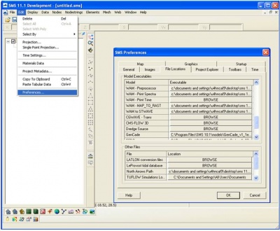
Once SMS 11.1 is open on the machine, it is necessary to specify the location of the GenCade executable. If this is specified incorrectly or not at all, GenCade will not run. In order to indicate the location of the executable, it is necessary to click on Edit, go to Preferences, and click on the tab labeled File Locations. The user should scroll down to GenCade under Model Executables and click on BROWSE. Once the GenCade executable is selected, the path for the executable should be listed under Model Executables next to GenCade. Figure 1 shows the File Locations window.
1.2 Set the Current Projection
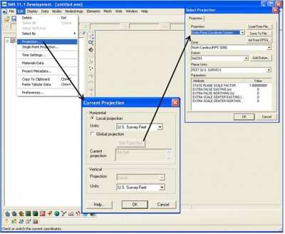
GenCade uses a real world coordinate system, so it is necessary to set up the current projection upon opening the SMS. GenCade projects may be set up in either U.S. customary units or SI units. The user may select the appropriate projection by clicking ‘’Edit->Projection’’. The steps to set up the projection are shown in Figure 2. This ensures all shorelines, structures, wave gauges, and other important features are mapped correctly. The user may also open aerial photographs to aid in completing the conceptual model. In many cases, the files representing shorelines and other features may be georeferenced correctly without defining the current projection; however, it is a good idea to define the projection before starting a GenCade project.
1.3 Reproject Current Projection
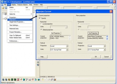
In some cases, an aerial photograph may be defined in a different coordinate system than the shorelines. It may also be necessary to develop the conceptual model for the GenCade project in a different coordinate system than the shorelines or aerial photos. In order to change the projection, the user should return to ‘’Edit->Project’’. The window will open, and the user can change the change the projection (Figure 3).
2. Preparing Input Files
2.1 Open and Define Initial Shoreline
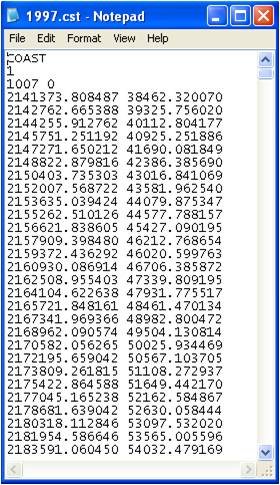
As mentioned previously, an initial shoreline is required to run GenCade. The model type must be defined as ‘’GenCade’’ before opening any file in the SMS. This can be accomplished by selecting ‘’Type->Models->GenCade ‘’ after right clicking on the default coverage under ‘’Map Data’’ in the data tree (panel on left side of screen). If the user has a file with a list of shoreline points that is in the same projection as the project, the file may be opened in the SMS. Before the file is opened in the SMS, it is important to double check the projection of coverage under ‘’Map Data’’. This can be done by right clicking on the coverage and clicking on Projection. If it is necessary to convert to a new projection for the shoreline, right click on the coverage and go to ‘’Reproject’’. A warning will pop up explaining that this is a non-reversible command; select ‘’Yes’’. Then a new window will open allowing the user to define the ‘’Current projection’’ and the ‘’New projection’’. To read the file into the conceptual model correctly, the file must be in *.cst format. The *.cst format requires the x and y coordinates of every point along the shoreline. An example of the format is shown in Figure 4. In order to modify a file with x and y coordinates for a shoreline, add the first three lines shown in Figure 4 which have been carried over from the old GENESIS format. The first number on the third line represents the total number of shoreline points listed in the file. This is the only number in the first three lines that will differ from the file shown in Figure 4.
There are many different ways to create an initial shoreline for GenCade in the SMS. If the shoreline is represented by points in a shapefile, these can be converted into a scatter set and saved as a text file. Then the text file can be modified to create the proper *.cst format and opened in the SMS.
A GenCade initial shoreline can also be created from a polyline shapefile. Once the shapefile is opened in the SMS, it is necessary to click on ‘’Mapping’’ and select ‘’Shapes->Feature Objects’’ (Figure 5). This will create a ‘’Feature Arc’’. After converting the ‘’Map Data’’ to ‘’GenCade’’, the arc may be selected by clicking on the ‘’Select Feature Arc’’ button and by double-clicking. If the shapefile was converted into multiple arcs, it is necessary to connect these segments to create one arc (Figure 6). Click on the ‘’Create Feature Arc’’ button and draw an arc connecting the existing arcs. Click on the ‘’Select Feature Point’’ button and select all of the nodes between the existing and the new arcs. To convert the nodes to vertices, go to ‘’Feature Objects’’ and select ‘’Vertices<->Nodes’’. Once all of the nodes have been converted to vertices, the shoreline is in the proper format for GenCade. When developing a shoreline in GenCade from a polyline shapefile, it is not necessary to create a *.cst file.
Regardless of whether or not the initial shoreline is opened as a *.cst file, the initial shoreline must be defined. To define the initial shoreline, ‘’GenCade’’ must be selected as the model type for the coverage. The feature arc representing the shoreline should be double-clicked (or right-click and select Attributes) after clicking on the ‘’Select Feature’’ Arc button. The ‘’GenCade Arc Attributes’’ window will open. The ‘’Initial Shoreline’’ option should be selected under ‘’Arc Options’’. These steps are shown in Figure 7.
2.2 Open and Define Regional Contour or Additional Shorelines
In some cases, a regional contour or additional shorelines may need to be added to the conceptual model. In order to define a second feature arc, it is necessary to right-click on ‘’Map Data’’ and select a ‘’New Coverage’’. This new coverage must also be defined as ‘’GenCade’’. The user can rename the new coverage, so that it can easily be identified. It is very important to open the new arc in a new coverage. If the arc is opened in the same coverage as the initial shoreline, the two arcs will most likely overlap, and the arcs will be split into many arcs. Once the regional contour is opened in the interface, define the arc as ‘’Regional Contour’’ in the ‘’GenCade Arc Attributes’’ window (Figure 8). A shoreline representing the final shoreline or an additional shoreline may be defined as a ‘’Reference Line’’.
2.3 Merge Coverages
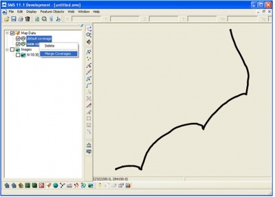
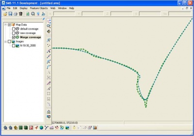
After the initial shoreline and regional contour have been loaded and defined in the SMS interface, it is necessary to merge the two lines in a single coverage. All structures, inlets, wave gages, and other features will be created in this single coverage. Highlight both the default coverage (initial shoreline) and the new coverage (regional contour). This can be done by hitting ctrl on the keyboard and clicking on both coverages. After right-clicking, select ‘’Merge Coverages’’. A window will open asking if the user would like to delete the coverages used to make the merged coverage. If no is selected, the initial shoreline and regional contour coverages will remain in the interface. It is a good idea to keep these coverages in the interface. If a problem occurs with the merged coverage, the initial shoreline and regional contour may be merged again. Figure 9 shows how coverages are merged while Figure 10 illustrates the initial shoreline and regional contour in the merged coverage.
3. Grid Setup
3.1 Create Inlets, Shoals, Dredging Events, and Jetties
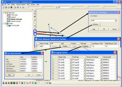
The inlet name, inlet shoal volumes, dredging events, and bypassing coefficients may be defined when an inlet is created. To do this, select the ‘’Create Feature Arc’’ button and draw a line from one side of the inlet to the other. When creating inlets and other features, a high quality aerial photo is very helpful. After the inlet is created, click on the ‘’Select Feature Arc’’ button and double-click on the arc representing the inlet. This can also be accomplished by a single click, followed by a right click. The ‘’GenCade Arc Attributes’’ window will open. Select ‘’Inlet’’ and click on ‘’Attributes’’. The ‘’Inlet Reservoir Model’’ window will open. The inlet can be named, shoal volume can be defined, and dredging events can be added. The initial and equilibrium shoal volumes for the ebb, flood, left bypass, left attachment, right bypass, and right attachment can be defined after clicking on the ‘’Volume’’ button. Similarly, after clicking on ‘’Dredging’’, the ‘’Dredging Events’’ window will open and the user can specify the beginning and ending date, the volume, and the shoal to be mined for each dredging event. The user also has the option to modify the left and right bypassing coefficients when jetties are present. Both the left and right bypassing coefficients have a default value of 1. Inlets that do not have jetties will not have a bypassing coefficient. After the inlet information is specified, the arc representing the inlet will turn blue. All of the steps create an inlet and add shoal volumes and dredging events are shown in Figure 11.
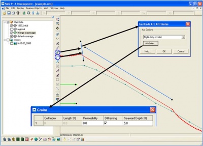
A jetty can be created at the inlet after selecting the ‘’Create Feature Arc’’ button. The arc representing the jetty should not intersect with the arc representing the inlet, regional contour, or initial shoreline. If this occurs, either the arc representing the jetty or the regional contour or initial shoreline will be split into two separate arcs. To remedy the problem of splitting arcs; the user should delete the arc representing the jetty, convert the newly created node to a vertex, and redefine the formerly split arc. After drawing the jetty, the user should click on the ‘’Select Feature Arc’’ and double-click on the line representing the jetty. When the ‘’GenCade Arc Attributes’’ window opens, the ‘’Left Jetty on Inlet’’ or ‘’Right Jetty on Inlet’’ should be selected. The left jetty is to the left of a person standing on land looking at the ocean. After ‘’Attributes’’ is selected, a new window will open where the ‘’Permeability’’ can be specified, ‘’Diffracting’’ can be checked or unchecked, and a seaward depth can be added. The default value for ‘’Permeability’’ is 0. Although ‘’Diffracting’’ is unchecked as a default option, the user should check this box in most cases. The line representing a jetty will also turn blue once all of required jetty information is provided. Figure 12 shows how to create a jetty.
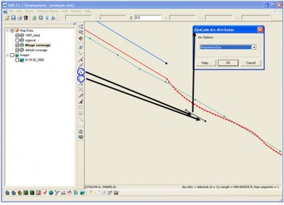
Once the grid is converted to GenCade, the bypassing bars associated with an inlet are defaulted to the one cell immediately adjacent to either side of the inlet. However, the bar size and location may be defined in the conceptual model. After the bar is created, it is necessary to double-click on the arc. Once the ‘’GenCade Arc Attributes’’ window is open, the bar can be defined as an ‘’Attachment Bar’’ (Figure 13). The attachment bar is also represented by a blue line.
3.2 Seawalls
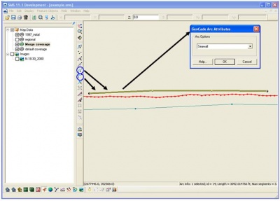
To draw a seawall, first the ‘’Create Feature Arc’’ button should be selected. The seawall must be drawn landward of the shoreline. If the user attempts to draw the seawall directly on top of the initial shoreline, an error will occur. The seawall drawn by the user should resemble the shape of the real seawall as closely as possible. If the user is not meticulous in drawing the seawall, the shape of the seawall in the GenCade model may not resemble the actual seawall. Additionally, since cell numbers are used in the GenCade model, the seawall shape may look different after converting from the conceptual model. After the seawall is drawn, the user should click on the Select Feature Arc button and click on the seawall. The ‘’GenCade Arc Attributes’’ window will open. ‘’Seawall’’ should be selected in ‘’Arc Options’’. The seawall will turn blue. When the model is converted to a 1D grid, an error message referring to the seawall may pop up. This message should be ignored; GenCade will modify the cells defined for the seawall. The user should review the seawall in the GenCade model. If the seawall does not resemble the actual seawall, the cell numbers and distances from the grid should be revised. A smaller cell size near the seawall may also be helpful. The process to create a seawall is shown in Figure 14.
3.3 Beach Fills
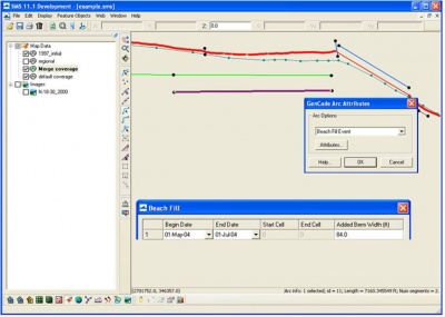
Beach fills can be created in the same way as inlets and seawalls. One should select the ‘’Create Feature Arc’’ button to draw the beach fill. Beach fills should be drawn slightly offshore. If there are many beach fills in one location during the simulation, draw the beach fills carefully so they do not connect or intersect. After each beach fill is drawn, click on the ‘’Select Feature Arc’’ and double-click on the line representing the beach fill. Select the ‘’Beach Fill Event’’ after the ‘’GenCade Arc Attributes’’ window opens. For each beach fill, add the ‘’Begin Date’’ and ‘’End Date’’ and the ‘’Added Berm Width’’. After selecting ‘’OK’’ in the ‘’GenCade Arc Attributes’’ window, the line representing the beach fill will turn green. Figure 15 demonstrates the steps to create and define beach fill events.
3.4 Detached Breakwaters
A detached breakwater is created by selecting the ‘’Create Feature Arc’’ button and drawing the arc representing the detached breakwater. The user should click on the ‘’Select Feature Arc’’ button and double-click on the detached breakwater. The ‘’GenCade Arc Attributes’’ window will open. Scroll down to ‘’Breakwater’’ and click on ‘’Attributes’’. The depth at each end of the detached breakwater can be entered in the ‘’Detached Breakwater’’ window. There is a pull-down window for wave transmission which includes constant transmission and three equations for time-dependent wave transmission: Ahrens, Seabrook and Hall, and d'Angremond.
3.4.1 Constant Transmission
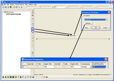
Under the ‘’Transmission’’ bar, select ‘’Constant’’. The last column in the detached breakwaters window is ‘’Coeff/Perm/Atts’’. For constant transmission, this represents the permeability of the detached breakwater. Once all necessary information is entered, click ‘’OK’’. The detached breakwater will turn orange. A detached breakwater with constant transmission is shown in Figure 16.
3.4.2 Time-dependent Wave Transmission
3.4.2.1 Ahrens
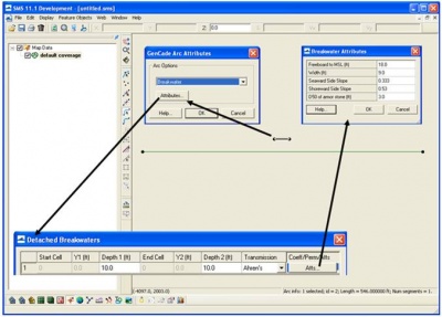
After selecting Ahrens under ‘’Transmission’’ in the ‘’Detached Breakwater’’ window, the final column (‘’Coeff/Perm/Atts’’) can be selected. Clicking this box will open the ‘’Breakwater Attributes’’ window. For Ahrens, the required values include freeboard to MSL, width, seaward side slope, shoreward side slope, and the D50 of the armor stone (Figure 17). Click ‘’OK’’, and the detached breakwater should turn orange.
3.4.2.2 d'Angremond
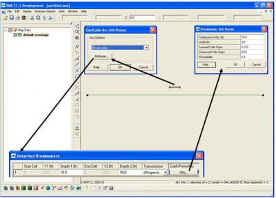
Another equation that can be used for time-dependent wave transmission is d'Angremond. Similarly to the option for ‘’Ahrens’’, click on the final column of the ‘’Detached Breakwaters’’ window which should now say ‘’Atts’’. For d'Angremond, the freeboard to MSL, width, seaward side slope, shoreward side slope, and permeability are required (Figure 18).
3.4.2.3 Seabrook and Hall
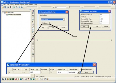
Seabrook and Hall can also be used for time-dependent wave transmission. After selecting Seabrook and Hall in the ‘’Detached Breakwaters’’ window, click on ‘’Atts’’ in the final column. The ‘’Breakwater Attributes’’ window will open, and the freeboard to MSL, width, seaward side slope, shoreward side slope, and D50 of the armor stone can be entered (Figure 19).
3.5 Groins
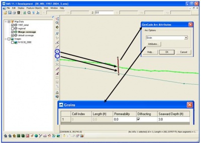
Once the location for a groin is chosen, select the ‘’Create Feature Arc’’ button. In many cases, the arc representing the groin will cross the regional contour and initial shoreline. Do not draw either end of the groin near the regional contour or initial shoreline. When this occurs, the node from the groin will connect to the initial shoreline or regional contour. This will divide the regional contour or initial shoreline into two separate arcs, where only one of the arcs will still be defined as the regional contour or initial shoreline. To remedy this, delete the arc that was created to represent the groin. Highlight the node that divides the initial shoreline into two segments. Under Feature ‘’Objects’’, select ‘’Vertices<->Nodes’’. The node will become a vertex, and the initial shoreline will once again be a single arc. After drawing the feature arc for the groin, click on the ‘’Select Feature Arc’’ button. The ‘’GenCade Arc Attributes’’ window will open. Select ‘’Groin’’ in the ‘’Arc Options’’ menu and click on ‘’Attributes’’. The window for groins is very similar to the window for jetties. The window for groins includes the ‘’Permeability’’ and ‘’Seaward Depth’’ (in the user specified units). The user may also define the groin as ‘’Diffracting’’ or ‘’Non-diffracting’’. When the ‘’Diffracting’’ option is checked, a ‘’Seaward Depth’’ must be specified. Figure 20 illustrates the various windows associated with creating a groin.
3.6 T-Groins
While a T-groin is not an arc attribute that can be created and defined in GenCade, a detached breakwater and a groin can be combined to form a T-groin. If a T-groin is required, the user should first create a detached breakwater and fill in all of the information necessary for a detached breakwater in the ‘’GenCade Arc Attributes’’ window. Then the user should create a groin that attaches to the detached breakwater. Once the conceptual model is converted to a 1D grid, it is necessary to double-check the T-groin to ensure that the shape has been retained. It is possible that the groin or detached breakwater has moved to an adjacent cell number and no longer retains the shape the user defined. The user may modify the cells for the detached breakwater or groin in the GenCade model under ‘’Edit Breakwaters’’ or ‘’Edit Groins’’ in the ‘’GenCade’’ menu. An example of a T-groin is shown in Figure 21.
3.7 Orientation, Cell Size, and Variable Grid Resolution
After defining the shorelines and any necessary structures, the grid should be set up. To manually draw the grid frame, click on the ‘’Create 1-D Grid Frame’’. The GenCade grid frame is purple and has an arrow at one end. If a person followed the grid from the end to the arrow, the water should always be to the left and the land should always be to the right. For example, if the GenCade grid was oriented from north to south, the water would be to the east (left) and the land would be to the west (right). The grid can be modified by clicking the ‘’Select 1-D Grid Frame’’ and double-clicking on the square in the center of the purple grid line. Alternately, the grid options can be changed by selecting the grid frame and right-clicking Properties. The ‘’Grid Frame Properties’’ window will open, and the ‘’Origin X’’, ‘’Origin Y’’, ‘’Angle’’, and ‘’I size’’ can be modified. The ‘’I size’’ is the length of the grid. ‘’Angle’’ refers to the sign convention in the conceptual model which is degrees counterclockwise from the x axis. This is different from the GenCade model convention (degrees clockwise from north). Therefore, once the map is converted to a 1D grid, the ‘’Azimuth’’ for the grid will be a different value. The cell size can be constant or variable. If the user chooses to change the cell size under ‘’Define cell sizes’’, the number of cells will change accordingly. The grid frame set up is shown in Figure 22.
A constant grid resolution is reasonable for most projects. However, there are some large scale projects that would benefit from variable grid resolution. Variable grid resolution can give more detail at specific locations of interest while having coarser resolution in other areas of the grid. By utilizing variable grid resolution, the simulation will run much more quickly than a grid with a constant, finer resolution. When the map is converted to a 1D grid, one of the options under ‘’I Cell Options’’ is ‘’Use refine points’’. This option refers to variable grid resolution.
First, it is necessary to determine which part of the grid needs a finer resolution. There are two ways to set up finer grid resolution. The user can decide to use one point or two points. For both of these options, click the ‘’Create Feature Point’’ button. If only one feature point is created, put the point at the location of interest. Click on the ‘’Select Feature Point’’ button and double-click on the point. The ‘’Refine Point’’ window will open (Figure 23). Check the ‘’Refine grid in I direction’’ and specify a base cell size. The base cell size is the size of the cells nearest to the refine point. This will be the smallest cell size in this location of the grid. Once the refine point is specified, right click on the coverage under ‘’Map Data’’ and convert ‘’Map->1D Grid’’. The ‘’Map->1D Grid’’ window will open (Figure 24). Under I Cell Options, click the button to specify the ‘’Use refine points’’ option. Type the maximum cell size and the maximum bias. The maximum cell size represents the largest cell size in the grid. Moving out from the one refine point, the cells will grow in size until a cell reaches the maximum cell size. The remaining cells in the grid will also be the maximum cell size. The maximum bias represents the amount each adjacent cell grows. For example, the default value is 1.10. This means each cell will grow 10%, so in a case with a base cell size of 10, the adjacent cells will have a size of 11. The cells will continue growing at this rate until a cell reaches the maximum cell size. In a case with only one refine point, do not select the ‘’Use inner growth’’ option.
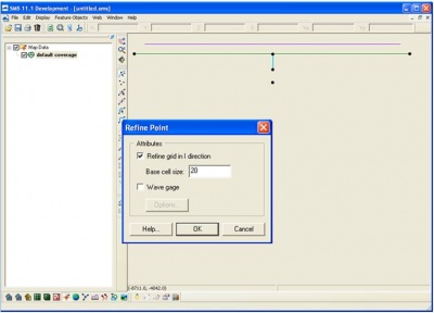
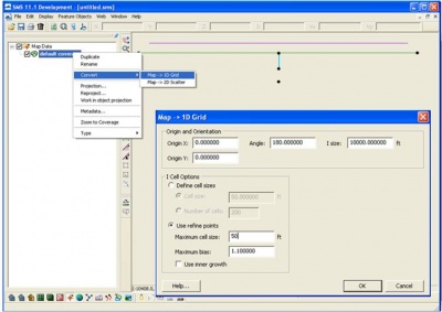
It is also possible to have a finer, constant resolution for a certain section within the grid. A groin field is a good example where a finer, constant resolution could be beneficial. For this case, select the ‘’Create Feature Point’’ button and create points on either side of the desired finer resolution area. Click on the ‘’Select Feature Point’’ button, double-click on each point, check the ‘’refine grid in I direction’’ option, and choose a base cell size (make this number the same for both refine points). Once again, convert to 1D grid and select the use refine points options. Follow the same procedure as the case with only one refine point for the maximum cell size and maximum bias. If the ‘’Use inner growth’’ option is left unchecked, the cells between each refine point will be constant (at the same cell size as specified for each refine point). The cells outside of the two refine points will continue to grow up to the specified maximum bias number. If the ‘’Use inner growth’’ option is selected, the cells will also grow between the two refine points. If the two refine points are close together, the cell size most likely will not reach the maximum cell size, but the cells between the two refine points will be larger than the base cell size.
Once the ‘’Use refine points’’ option is chosen in the ‘’Map->1D Grid’’ window, the resulting GenCade grid will have variable resolution. After saving the project, the *.shdx file is also created. This file lists the size of each cell in the grid. This file is needed to make shoreline change or transport plots outside of SMS in cases where variable grid resolution is utilized.
3.8 Convert to 1-D Grid
Once all of the shorelines, inlets, structures, and refine points have been added to the conceptual model, select the merged coverage, right click on the name, click on ‘’Convert’’, and select’’ Map->1D Grid’’ (Figure 25). A window will open showing the origin and orientation of the GenCade grid and the different cell options. This is the same window that was opened when the grid frame was created. Once the map has been converted to a 1D grid, the data tree in the SMS will show ‘’GenCade Data’’ and ‘’GenCade Grid’’. If the user highlights ‘’GenCade Data’’, the GenCade menu at the top of the interface will appear. The newly developed GenCade grid can be seen in the viewing window.
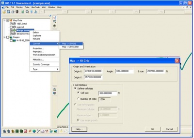
3.9 Wave Data
Wave gauges should be defined after converting from the conceptual model to the GenCade model. After the GenCade grid has been created, highlight the coverage under ‘’Map Data’’ to return to the conceptual model. Wave gauge data may be entered in GenCade in four conventions: shore normal, meteorological, oceanographic, and cartesian. Regardless of the convention, wave directions will be converted to shore normal convention in the *.wave files. Therefore, the grid must be created first, so that GenCade can convert the wave directions to shore normal.
There are two ways to represent wave gauges in the conceptual model. In both cases, the user needs to create and select the feature point. If the coordinates of the wave gauges are in the same coordinate system as the conceptual model, it is very easy to create a point at the location of each gauge. Drag the file with the coordinates representing the wave gauges into the SMS interface. The ‘’Open File Format’’ window will open. Select ‘’Use Import Wizard’’ and click ‘’OK’’. Follow the directions for the ‘’File Import Wizard’’ and select ‘’OK’’. The wave gauges will be represented as scatter data. Simply select the ‘’Create Feature Point’’ button in the conceptual model and draw a feature point directly on top of each point. Now the wave gauge locations are represented in the conceptual model. Instead of defining the feature point as a refine point, check ‘’Wave Gage’’. The ‘’Options’’ button will open a window where the water depth may be defined. Click on ‘’Data’’ to open the ‘’Wave Events’’ window (Figure 26). This window will allow the user to copy and paste data or import the wave information from a text file. Regardless of the format of the wave information, the user first needs to define the coordinate convention under ‘’Angle Settings’’. Depending on the source, the wave information will likely be in meteorological and oceanographic convention.
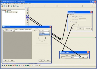
Before importing the wave information, double check to make sure there is no missing or incorrect data. In previous versions of the interface, the SMS could not handle wave directions from land; however, this has been corrected.
If the wave information is in Microsoft Excel or a similar format, it may be easiest to directly copy and paste. There are four columns of information necessary to paste the data correctly (Figure 27). The first column represents the date (month, day, year, and time), the second is the wave height, the third column is the wave period, and the fourth column is wave direction. The date must be in MM/DD/YYYY HH:MM format. Regardless of the units used in the conceptual model, Ho must be in meters. The reason the grid must be created before adding the wave information is due to the shore normal convention. To convert from any convention to shore normal, the SMS must know the angle of the shore (grid). When the wave directions are in shore normal convention, it is important to note that the conceptual model and GenCade model use different sign conventions. To import the correct wave directions in shore normal coordinates, the user should go to ‘’GenCade->Edit Grid’’ when in the GenCade Model. The ‘’Azimuth’’ is the correct angle to determine shore normal coordinates. The ‘’Angle’’ in the ‘’Grid Frame Properties’’ window will list a different value since the sign convention for the conceptual model is different from the GenCade model. If the value for ‘’Angle’’ is used to determine shore normal coordinates, the wave directions will be incorrect. If the wave information pasted into the ‘’Wave Events’’ window was in meteorological, oceanographic, or cartesian convention, the user must change the ‘’Projection’’ under ‘’Angle Settings’’ to ‘’Shore Normal’’. If the user does not convert to ‘’Shore Normal’’ at this point and immediately converts to the 1D grid, the direction of the waves will be converted incorrectly. After changing to ‘’Shore Normal’’ in the ‘’Wave Events’’ window, the user should double-check that the conversion is correct.
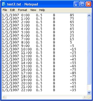
A second way to enter the wave information is by clicking ‘’Import’’ at the bottom of the ‘’Wave Events’’ window. The ‘’Import’’ function allows the user to find the text file with the wave information. Text files must have five columns representing the wave information (Figure 28). The last three columns are in the same format as the copy and paste option (wave height, wave period, and wave direction). The first column lists the date in YYYYMMDD format. The second column lists the time in HHMM format. Once the file is read by the SMS, each column must be identified (Figures 29 and 30). Once ‘’Finish’’ is clicked, a ‘’Direction Angle Convention’’ window should open. The angle convention should be the same as the projection identified under ‘’Angle Settings’’. After pushing ‘’OK’’, the wave information should be in the proper format under ‘’Wave Events’’. Before closing the ‘’Wave Events’’ window, remember to change the projection to ‘’Shore Normal’’ if the waves were originally in meteorological or oceanographic convention (Figure 31). The wave directions should change accordingly. If the wave imported were already in shore normal convention, this step is not necessary. Once all of the wave gauges are populated, the user may convert to the 1D grid.
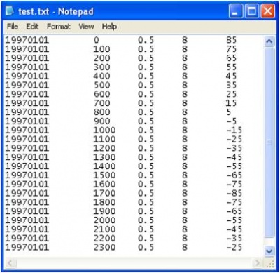
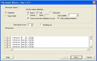
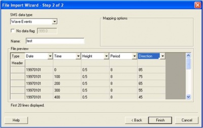
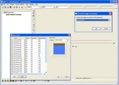
4. GenCade Files, Menu, Model Setup, and Execution
4.1 GenCade Input Files
There are three input files required to run GenCade. The GenCade control file (*.gen) lists all information related to the GenCade simulation. This file records the details for structures, inlets, dredging events, beach fills, boundary conditions, wave gauges, and the model setup. This file also defines the paths for each of the input files and one of the output files, the *.prt file. Although the *.gen file can be opened, it is recommended that the user refrain from making any changes. The initial shoreline (*.shi) and wave file(s) (*.wave) are also necessary to run even the simplest GenCade simulations. A separate wave file is created for each wave gauge. The regional contour file (*.shr), water level file (*.wl), and variable resolution file (*.shdx) are optional input files. The water level file is only created when time-dependent wave transmission is necessary.
4.2 GenCade Menu
Once the conceptual model is converted to the 1D grid, the ‘’GenCade’’ menu will appear between ‘’Data’’ and ‘’Web’’ in the menu bar (Figure 32). This menu can be used to make minor changes to the project and to double-check that all features defined in the conceptual model are represented in the grid. An example of a minor change to make in the GenCade model is modifying the cells representing the left and right bypassing under the ‘’Edit Inlets’’ menu. If the user is calibrating the model, it is best to return to the conceptual model to make any changes. Changes made in the conceptual model may be applied to multiple projects, but changes made to the grid itself cannot.
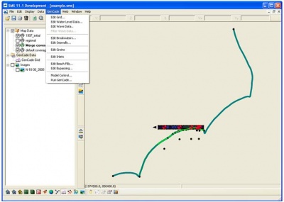
4.3 GenCade Model Setup
Once the user has determined that all of the features defined in the conceptual model have been retained in the GenCade grid, the user should begin to set up the model. This is accomplished by selecting ‘’Model Control’’ under the ‘’GenCade’’ menu. The first tab in the ‘’GenCade Model Control’’ window is the ‘’Model Setup’’ (Figure 33). It is in this window that the user may specify the starting and ending date of the simulation, the time step, and the recording time step. The simulation time step must be equal to or less than the wave time step. If the wave time step is smaller than the simulation time step, an error will occur and GenCade will not run. The default time step is 1.0 hour, and the default recording time step is 168.0 hours. The user may also give the simulation a title. The bottom right of the menu states ‘’Print Dates’’. In some cases, the user may be interested in the shoreline at a specific date not normally written in the print file (shoreline and transport information are only recorded yearly). Additional dates of interest may be added under ‘’Print Dates’’.
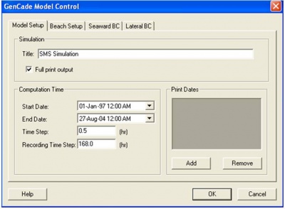
4.4 Beach Setup
The second tab under ‘’GenCade Model Control’’ is the ‘’Beach Setup’’ tab (Figure 34). The first section under this tab refers to the ‘’Sand and Beach Data’’. Here the user may enter the ‘’Effective Grain Size’’ (always in mm), the ‘’Average Berm Height’’, and the ‘’Closure Depth’’. The default ‘’Effective Grain Size’’ is 0.2 mm. Depending on the specified units, the default ‘’Average Berm Height’’ is 1.0 ft or 1.0 m and the default ‘’Closure Depth’’ is 10.0 ft or 10.0 m. ‘’Longshore Sand Transport Calibration Coefficients’’ can also be found under ‘’Beach Setup’’. The defaults values for ‘’K1’’ and ‘’K2’’ are 0.5 and 0.25, respectively. These values should be adjusted during the calibration process.
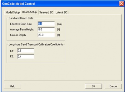
4.5 Seaward BC
The next tab under ‘’GenCade Model Control’’ is the ‘’Seaward BC’’ (or Boundary Condition) tab (Figure 35). The two main options in this tab are the ‘’Input Wave Adjustments’’ section and the ‘’Other Options’’ section. Under ‘’Input Wave Adjustments’’, the user may modify the ‘’Height Amplification Factor’’, ‘’Angle Amplification Factor’’, and ‘’Angle Offset’’. In the ‘’Other Options’’ section, the user may define the ‘’Number of Cells in Offshore Contour Smoothing Window’’. The default ‘’ISMOOTH’’ value is 11, but it is suggested that this number range between 11 and 101. This is another value that must be adjusted during the calibration stage.
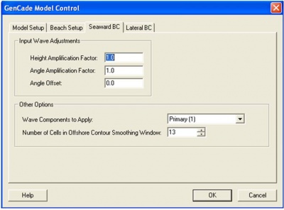
4.6 Lateral BC
The final tab under ‘’GenCade Model Control’’ is the ‘’Lateral BC’’ (or Boundary Condition) tab. There are three options for the ‘’Left Lateral BC’’ and ‘’Right Lateral BC’’: Pinned, Gated, and Moving.
4.6.1 Pinned Boundary Condition
The pinned boundary condition is the default and should be used in most cases. A boundary specified as pinned will not move from the initial shoreline. When the pinned boundary condition is selected, all other options under ‘’Lateral BC’’ will be grayed out. The pinned lateral boundary condition is shown in Figure 36.
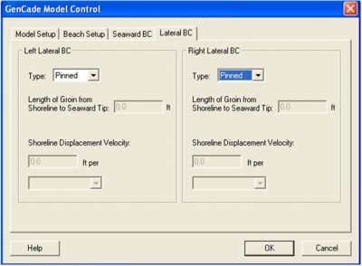
4.6.2 Moving Boundary Condition
If a moving boundary condition is selected (Figure 37), the boundary will move a certain distance over a time period entered by the user. When a moving boundary is selected, the ‘’Length of Groin from Shoreline to Seaward Tip’’ will still be grayed out, but the ‘’Shoreline Displacement Velocity’’ will be active. Under ‘’Shoreline Displacement Velocity’’, the user should enter the shoreline displacement in the same units used to set up the grid. This shoreline displacement may occur over the entire simulation period, a day, or a time step. Shoreline displacement over the entire simulation is the most common input for a moving boundary condition, because many users have shorelines for the beginning and end of a simulation. If the user chooses to specify the shoreline displacement per time step, it should be noted that this number should be very small. For example, in an example with a time step of 0.5 hr and a shoreline displacement of 0.5 ft per time step, the total shoreline displacement during a two year simulation would be 17,520 ft.
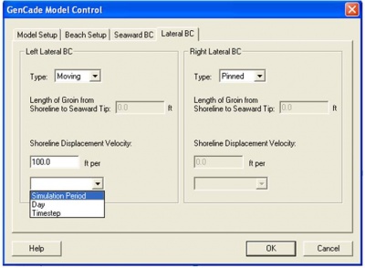
4.6.3 Gated Boundary Condition
The final boundary condition available in GenCade is a gated boundary condition (Figure 38). A gated boundary condition is bounded with a groin, so this is beneficial in cases where a groin or a jetty is located near the boundary. In the case of a gated boundary condition, it is also necessary to create and define a groin at the left or right boundary in the conceptual model. If the right lateral boundary is defined as a gated boundary, the groin should have a cell number of N+1. For example, if the grid has 100 cells, the groin should be located at cell number 101. After a gated boundary condition is selected, the ‘’Length of Groin from Shoreline to Seaward Tip’’ will be active.
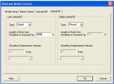
4.7 Running GenCade
Once the GenCade grid and all of the parameters in ‘’Model Control’’ have been updated, it is possible to run GenCade. Please remember to save the project before running GenCade. If the project is not saved prior to running GenCade, the most recent additions to the grid will not be written in the *.gen file. To run GenCade, go to the ‘’GenCade’’ menu and select ‘’Run GenCade’’ (Figure 39). A window will open that will describe the simulation. This window will notify the user if an error has occurred. Although there is no time bar stating the amount of time left in the simulation, the window will show when GenCade has finished calculating each year in the time simulation. The window will alert the user when the model is finished and will prompt to exit. Generally, it does not take very long to run GenCade. For an example with a 300 ft cell size, 635 cells, and a time step of 0.1 hour, it takes only about a minute to run each year of the simulation. A smaller cell size will significantly slow down the simulation, but it should still take less than 10 minutes to run for each year in the simulation. Multiple inlets, dredging events, and beach fill can also increase the run time.
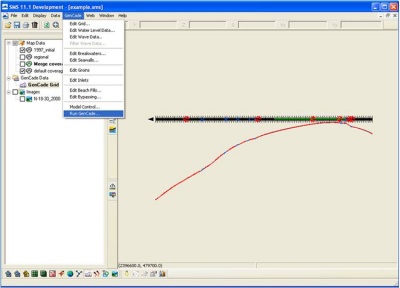
4.8 GenCade Output Files
Following a GenCade simulation, at least seven output files will be created in the assigned directory. The print file (*.prt) saves all of the information related to the simulation including wave heights, shorelines, and transport rates. The shoreline position output file (*.slo) documents the shoreline position for each time step for every cell in the grid. The net transport rate file (*.qtr) prints the net transport rate for each cell at every time step. The inlet shoal volume file (*.irv) lists volumes for each inlet shoal for every time step. A separate inlet shoal volume file is created for each inlet represented in the simulation. If the grid does not include an inlet, the *.irv file will not be created. All of the files except the print file may be opened and viewed in the SMS. The aforementioned files contain the majority of the information a user would need to evaluate the results of a simulation. The mean net annual transport files (*.mqn [mean annual net transport], *.mql [mean transport to the left], and *.mqr [mean transport to the right]) list the transport for each cell for each time step. The offshore contour for each time step for each cell is included in the offshore contour file (*.off). Additional information about GenCade output files can be found here.
4.9 Visualizing Results
Following a simulation, several output files will be created. These were listed in Table 1. Many of these files may be opened in the SMS for visualization. The first of these files is the *.slo file, or shoreline change file. Once this file is opened in the SMS, a box with the header ‘’Time Steps’’ will appear. An arc representing the calculated shoreline should appear in the grid window. The default color and size of the calculated shoreline may be difficult to view. Go to ‘’Display->Display Options’’ and click on ‘’1D Grid’’ to change the size and color of the calculated shoreline (Figure 40). The size and color of the initial shoreline, regional contour, and structures can also be changed. The default time under ‘’Time Steps’’ is ‘’Relative Time’’. To view the simulated dates, right click on the words ‘’Time Steps’’ and select ‘’Time Settings’’. Change the zero time to represent the first date in the simulation. Under ‘’Time Display’’, change ‘’Relative Time’’ to ‘’Absolute Time/Date’’. The user can view the calculated shoreline at any date during the simulation and compare it with the initial shoreline or other reference line (Figure 41).
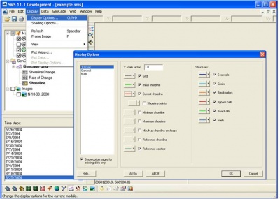
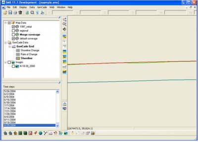
Plots can also be viewed in SMS. Under ‘’Display’’, click on ‘’Plot Wizard’’ (Figure 42). In the first window, select ‘’GenCade Shoreline’’ as the plot type. Keep the ‘’Active dataset’’ under ‘’Dataset’’ and ‘’Active time step’’ under ‘’Time step’’ selected and click ‘’Finish’’. A new window will appear showing the shoreline for the selected time step (Figure 43). Once the plot has been created, simply highlight ‘’Rate of Change’’ or ‘’Shoreline’’ under ‘’GenCade Grid’’ in the data tree to change the plot.
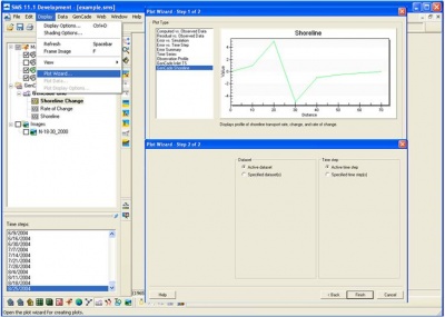
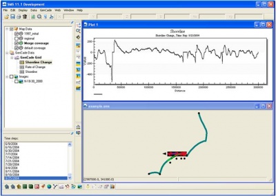
The inlet shoal volumes over the entire simulation may also be viewed in the SMS. Go to ‘’Display’’ to ‘’Plot Wizard’’. Under ‘’Plot Type’’, select ‘’GenCade Inlet TS’’ and click ‘’Next’’ (Figure 44). The user may select any of the inlets included in the project and may choose the entire simulation or only a few years. The user may select one shoal or many shoals. After selecting the inlet, time, and corresponding shoals, click ‘’Finish’’. A new window with the shoal volumes over the course of the selected dates will open (Figure 45).
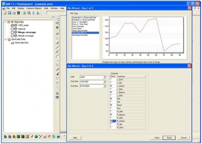
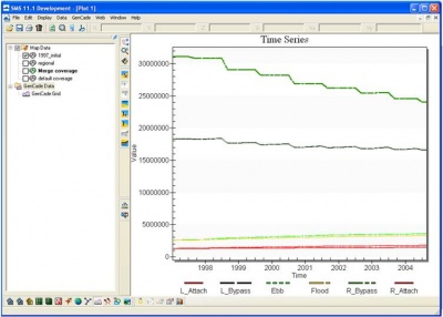
Some users may want to plot shoreline change in Microsoft Excel or similar software. All of the information collected during the simulation was saved in the *.prt file (Figure 46). The shoreline change after each year in the simulation is located in this file. Although the shoreline change is not in column format, the format can easily be changed with a simple code. If the case uses constant resolution, the size of each cell is known and this information can easily be added to a spreadsheet. In the case of variable resolution, there is an additional input file: *.shdx. Each number in this file represents the grid cell size. The numbers in the file can also be converted to column format. Once the distance alongshore and the shoreline change have been added to Microsoft Excel or other spreadsheet software, then the shoreline change can be plotted.
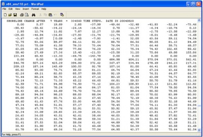
It is also possible to use Microsoft Excel to plot longshore transport. In the *.prt file, longshore transport can be found by searching for ‘’“mean net annual transport”’’. This section of the *.prt file is shown in Figure 47. Please make a note of the units for transport listed in the *.prt file. The longshore transport can be plotted in Microsoft Excel in the same way as shoreline change.
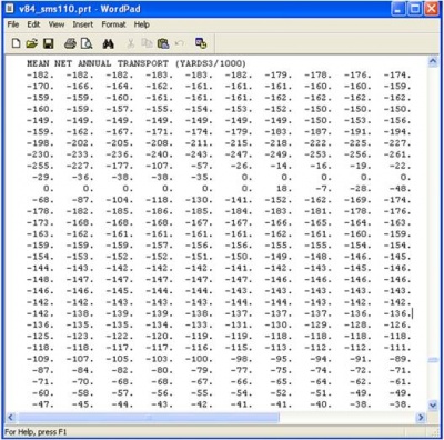
It is slightly more difficult to compare the calculated shoreline to a measured shoreline. First, save as a new project. Open the measured shoreline in the SMS and define it as the initial shoreline (for this new saved project). Convert to 1-D grid again and save as a new project. This will save the measured shoreline as the initial shoreline. Both the measured and calculated shoreline will need to be compared to the initial shoreline. The values in the *.shi file represent the distance from the initial shoreline to the grid for each cell. The calculated shoreline can be found in the *.prt by searching for shoreline position after the total number of years in the simulation. These numbers will represent the distance offset from the GenCade grid. Shoreline change after each year in the simulation can also be found in the *.prt file. By saving the measured shoreline as the initial shoreline, this allows SMS to produce an input file for this shoreline in the same format as the initial shoreline and calculated shoreline. All of these shorelines can be converted to column format and pasted into Microsoft Excel. Subtract the initial shoreline from the measured shoreline and the calculated shoreline to get shoreline change for the measured and calculated shorelines.
5. Developing Alternatives
There are several reasons that a user may need to modify a GenCade grid. While calibrating the model, it may be necessary to refine the grid. Some examples of modifications necessary to develop alternatives include changing a small section of the regional contour, changing the initial shoreline, or adding new structures.
5.1 Minor Changes to the Regional Contour or Initial Shoreline
After setting up and running the model and looking at results, it may become necessary to make a minor modification to the regional contour or initial shoreline. For example, the initial shoreline may need to be smoothed near an unstructured inlet or the regional contour may need to be adjusted to account for a large ebb shoal.
To make changes to the regional contour or initial shoreline, return to the merged coverage with all of the shorelines, structures, and wave gauges under ‘’Map Data’’. Click ‘’Select Feature Vertex’’ and drag each vertex to the desired location (Figure 48). It is also possible to add vertices by clicking ‘’Create Feature Vertex’’, adding the vertex, and moving it to the selected location. Extra vertices can be deleted after they are selected. Once the required updates to the regional contour or the initial shoreline are made, right click on the merged coverage and convert ‘’Map->1D Grid’’. The initial shoreline or regional contour must be selected by clicking on the ‘’Select Feature Arc’’. If the arc is not selected and highlighted, the old regional contour or initial shoreline will not be replaced. It should also be mentioned that only minor changes should be made to the regional contour or initial shoreline. The user should not modify the regional contour during model calibration.
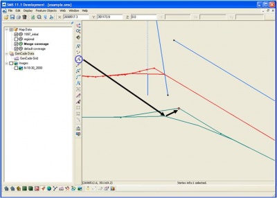
5.2 Modify Existing Structures or Beach Fills
For some alternatives, a beach fill or structure may need to be extended. To extend a structure, click on ‘’Select Feature Point’’. Click on the node at the end of the structure and extend it to the desired length. Beach fills can be modified in the same way. Right click on the merged coverage and convert ‘’Map->1D Grid’’. The modified structure must be selected (by clicking on ‘’Select Feature Point’’) for the changes to be noted in the GenCade model.
5.3 Replace Initial Shoreline or Regional Contour
Some projects may require analysis for several different time periods. If the structures exist during multiple time periods and the wave gauge data span many decades, it may be easiest to replace the initial shoreline in the conceptual model. The same process can be used if a new regional contour is necessary. Do not delete the existing GenCade grid. Right click on ‘’Map Data’’, click ‘’New Coverage’’, and select ‘’GenCade’’. It is best to give the new coverage a specific name that can be identified easily. Right click on this new coverage and scroll down to ‘’Type->Models->GenCade’’. Open the new shoreline or regional contour in the new coverage. Click on ‘’Select Feature Arc’’ and define the arc. Right click on the new coverage and convert ‘’Map->1D Grid’’. The new initial shoreline or regional contour will replace the original.
5.4 Add Structures or Beach Fills
When a project has many different alternatives, it may be necessary to add new structures. Instead of developing a new grid for each alternative, features can be modified or added to a base grid that already has the initial shoreline, regional contour, wave gauges, and basic structures and beach fills. Right click on ‘’Map Data’’ and select ‘’GenCade’’ under ‘’New Coverage’’. Right click on this coverage and confirm that the model type is ‘’GenCade’’. In this new coverage, add new structures and beach fills by selecting the ‘’Create Feature Arc’’ button. Specify the type of arc. Once all the new structures are included, right click on the new coverage and convert ‘’Map->1D Grid’’. The new arcs will be added in the GenCade grid. Additional structures or beach fills can also be added directly to the merged coverage that already has the initial shoreline, regional contour, and existing structures.
5.5 Modify Wave Gauges
The instructions above regarding adding new features can also apply to adding new wave gauges. However, sometimes the wave gauge data need to be modified. In reviewing the wave gauge information, a user may find that a few of the dates or values may be incorrect. If only a few values need to be modified, click on the merged coverage and select the wave gauge by clicking on ‘’Select Feature Point’’ and double-click on the point representing the wave gauge. Click on ‘’Options’’ and click on ‘’Data’’. Manually update the incorrect wave information. Once finished, convert ‘’Map->1D Grid’’. The wave gauge will now include the correct wave information. The steps to modify a wave gauge are shown in Figure 49.
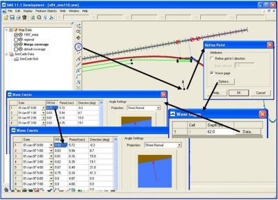
A user may also determine that an entire set of wave gauge information may be incorrect. This can occur by selecting the wrong wave gauge when pasting values or by incorrectly manually transforming waves. This can be remedied by deleting the existing wave gauge, creating a new wave gauge, and following the steps to add information to the wave gauge.