TAPtides

Tidal Analysis and Prediction of Tides: TAPtides

By John D. Boon and Alejandro Sanchez

Purpose

The Coastal Inlets Research Program Technical Wiki herein describes the desktop computer program TAPtides for the Tidal Analysis and Prediction of water levels. Designed to be easy to use, its Graphical User Interface (GUI) permits quick separation of a time series of water level measurements into its tidal and non-tidal components using a selective least squares harmonic reduction employing up to 35 tidal constituents. After saving the tidal constants for the constituents selected during analysis, the user can generate predictions of the astronomical tide, the water level that varies at known tidal frequencies attributable to gravitational interactions between the earth, moon, and sun.

Introduction

Many software packages are available today that allow tide predictions to be made in tidal waterways throughout the world. With few exceptions, these programs use tidal constants determined by governmental agencies and the casual user of this software is generally unaware of any of the details involved in the analysis, not least the breakdown of observed water level variation into its tidal and non-tidal parts.

In many cases, little information is available to users on the length, quality or age of the water level time series used to estimate tidal constants. Predictions for coastal waterways that have undergone significant hydrologic change (storms, dredging activity) may be subject to errors resulting from outdated measurements. The software presented here gives users the ability to make tidal harmonic predictions where suitable data are available for calculating the tidal harmonic constituents.

TAPtides is the ideal package to explore and develop preliminary or finalized tidal predictions from serial records spanning several weeks to several months. Although its operating features are intuitive and can be quickly grasped by users familiar with MS Windows^® terminology, it is important to have a general understanding of the theory of tides before using TAPtides. Comprehensive references such as Cartwright (2000) and Pugh (2004) are highly recommended for this purpose, as is Boon (2004) for a practical introduction.

Installation

To run TAPtides the MATLAB Component Runtime (MCR) program must first be installed using the MCRInstaller provided with the application package. When installing SMS select the option to install TAPtides and TAPcurrents. After unzipping the package in a working directory, right-click the TAPtides program icon to create a shortcut and place it on your desktop. Run the application by double-clicking on the icon: This will create a new folder with the required MCR programs. TAPtides is programmed in the MATLAB^® technical computing language, a product of The MathWorks, Inc. The present program is compatible personal computers with the MS Windows operating system (Windows XP).

Overview

The TAPtides menu has two options Tidal Analysis and Tidal Prediction. The last two buttons launch programs to conduct water level analysis (TIDAL ANALYSIS) and generate tide predictions respectively (CHOOSING TIDAL CONSTITUENTS, TIDAL PREDICTION). The analysis portion of the software accepts several file types (see INPUT FILES). The files used in this CHETN are automatically downloaded during the installation process and are located within the TAPtides folder which is located in the SMS directory. The tidal prediction portion of the software requires tidal constituents (amplitudes and phases of individual tidal components) from the tidal analysis program.

Tidal Analysis

Figure 1. TAPtides Analysis Page.

The method used by TAPtides to analyze a water level time series is commonly known as Harmonic Analysis, Method of Least Squares (HAMELS). It achieves a progressive reduction in variance (mean square deviation about the mean) by adding harmonic terms with specific astronomical frequencies to a general least squares model of the type used for multiple regression. It is not Fourier analysis, a procedure that employs only the Fourier frequencies. A brief description of HAMELS is given in Appendix B. For a complete description of the least squares harmonic analysis method employed here, the reader is referred to Boon (2004).

It is preferable to use the term water level analysis, rather than tide analysis, because the measured change in water level in coastal waterways varies at both tidal and non-tidal frequencies, including frequencies so low they appear as a static level or linear trend in short series. The objective of the analysis is to separate these components so that a tidal height prediction can be made with the component that is predictable – the water level that oscillates at tidal frequencies. To perform a water level harmonic analysis, click on the ’</nowki>Tidal Analysis<nowiki>’ button within the TAPtides window.

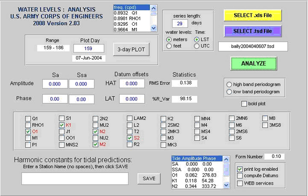
Clicking the Tidal Analysis button within the SMS menu Tools|Harmonic Analysis starts the GUI page that performs tide analysis (see Figure 1). It is recommended that the user click on the Disclaimer menu at the top of the window and read the disclaimer message before proceeding. Click the Program Help menu immediately to the left of the Disclaimer button to view information about input files, file analysis, selection of tidal constituents and other topics.

The analysis occurs in two steps:

1. Settings and File Selection: Enter time series length (in days) and water level units (meters or feet). If the series length is left empty the total duration of the imported file will be used. If a number is entered that is larger than the input series length, a warning message will occur and the series length will be reduced automatically. Select a data file for analysis using the appropriate press button in the upper right corner of the page. Pressing a button will open a file browser displaying only files of the indicated type (MS Excel files with .xls extension or ascii text files with .tsd extension). Select a file and press the open button in the browser. If the print log enabled box is checked, a text file will be generated containing the parameters selected and other information from the analysis.
2. Analysis: After the file is loaded, the message File ready for analysis will appear in the data box directly below the file selection buttons and the large Analyze button will turn green Pressing the ANALYZE button will start the analysis. The number of days in the file selected will be briefly displayed in the data box, followed by the date and time of the first record in the file and the file name. A graph will appear next showing the results of a least squares harmonic analysis fitting the five main tidal constituents, O1, K1, N2, M2 and S2, to the water level data (Figure 2). A list box at the bottom of the page displays the tidal constants (amplitude and phase) computed for all five constituents.

The check boxes in the center of the window indicate the tidal constituents available for harmonic analysis. Initially, only five major constituents are activated (shown in red text). The first five are always selected but the thirty others should be thought of as potential constituents that may be included in subsequent rounds of analysis. To include additional constituents, click on the check boxes for individual constituents and press the ANALYZE button. Selecting the proper constituents is explained in the next section.

For a relatively short time series of water levels (29 days to 58 days), there are limits to the number of constituents that can be used in a harmonic analysis. In general, the difficulty caused by short time series arises from the resolution of certain constituents that are close to others in frequency (consult the list box at the top of the Analysis page for a list of available constituents and their frequency). The main solar semidiurnal constituent S2, for example, has a frequency of exactly 2 cycles per mean solar day (cpd); the semidiurnal constituents T2 (1.9973 cpd), R2 (2.0027 cpd) and K2 (2.0055 cpd) are all very close to this frequency and can be difficult to resolve from a short series. The minimum series duration T necessary to fully resolve two tidal frequencies f₁ and f₂ is given by T =1/|f₁-f₂|, the synodic period. The synodic period for S2 and K2, for example, is 1/0.0055 or 181.8 days. Another important aspect to consider is the number of constituents chosen to model the tide. The user should start with the default constituents and choose additional constituents on the basis of their ability to reduce residual variance without violating the synodic period rule. Likely candidates will be found using the high band periodogram to examine the total distribution of variance (energy) with frequency. The periodogram feature is further explained below.

Three-day Plot

During analysis, the three-day plot feature in the gray frame on the upper left side of the TAPtides window may be used to closely examine three-day periods of the time series. Like the main plot which appears after pressing the ANALYZE button, the 3-day plot uses Julian days to display time (the corresponding calendar date is also displayed for convenience). The three-day plot of observed (red), predicted (blue) and residual (green) water level gives a wave-by-wave view showing how well the tidal harmonic model fits the data. A flat residual line indicates a good fit. If the predicted (blue) curve shows double peaks where the observed (red) curve only has single peaks, this may be an indication that too many tidal constituents are being used.

Another good reason to use the three-day plot is to investigate errors; e.g., dropped data points, vertical datum shift, or a shift to incorrect times. The least squares algorithm used in TAPtides is not affected by small data gaps (provided the time stamping remains correct). Although a short gap may be acceptable, the program will still issue a warning if the number of observations found is less than the number expected based on the series length specified and the calculated sampling rate based on the first two recorded sample times in the data series.

Additional Tools

Several tools are provided to assist the user in choosing constituents for inclusion in a harmonic model of the astronomical tide. Rather than relying on any single one of these tools, the user should use them in combination while keeping the series length in mind. Following a brief description of the available tools listed below, two examples of the recommended tidal analysis procedure are presented to illustrate their use.

Residual Periodogram

The residual periodogram is a line spectrum depicting the distribution of residual (measured minus predicted) energy at the Fourier frequencies. Fourier frequencies are multiples of the fundamental frequency 1/T and thus may not coincide with the tidal frequencies which, with the exception of the overtides (S4, S6, M4, M6, M8), are not multiples of any given frequency. However, with increasing series length Fourier frequencies become more numerous and bandwidth decreases, resulting in closer approximations to tidal frequencies. Using the data cursor in the MATLAB figure containing the high band periodogram (1-8 cpd), the user can determine the frequencies associated with the highest spectral peaks and look for the closest match to one of the tidal frequencies shown in the list box at the top of the analysis page, checking the appropriate box for the constituent indicated. At this point the user should consider each new constituent as only a candidate for inclusion in the tidal model, to be verified in subsequent analysis. Note that much of the residual variance displayed in any one periodogram may well be due to non-tidal meteorological forcing.

For convenience, both a high band periodogram (1 to 8 cpd) and a low band periodogram (0 to 3 cpd) are provided. The high band periodogram is well-suited for examining intertidal energy associated with transient events (e.g., storm surge). The low band feature can be used to examine subtidal oscillations that are usually associated with low frequency extratropical forcing. Subtidal energy (variance) in particular can be large compared to the tidal energy at certain locations. In those instances harmonic analysis will account for a low percentage of the total variance regardless of the number of tidal constituents used. Likewise the harmonic model of the tide cannot be deemed to have "failed" for this reason since it is designed to predict only the water level change occurring at tidal frequencies.

RMS Error and Percent Reduction in Variance

Two statistical parameters are provided near the center of the Analysis window to assist the user in evaluating the degree of success achieved by the model in representing the data. The RMS error, calculated as the square root of the mean square difference between observed and predicted water levels, is a measure of the expected error associated with an individual water level prediction. The Percent Reduction in Variance (%R_Var) is the percentage of the total variance in water level explained by the astronomical tide model. Ideally, inclusion in the model of any one constituent suggested by the periodogram should result in a noticeable decrease in RMS error combined with an increase in %R_Var. Again, if the data are taken from a region with strong meteorological forcing in relation to the tidal regime, it will not be possible to achieve either a high %R_Var or a low RMS error.

Constituent Amplitude and Phase Estimates

After conducting an analysis with a new tidal constituent added to the model, the user should check the amplitude found for that constituent in the list box at the bottom of the Analysis window. It should exceed at least one percent of the largest major constituent amplitude. More importantly for a short series, it should not cause another constituent at an adjacent frequency to change either its amplitude or phase by more than a few percent (K2 and S2 may be exceptions). When this occurs, it indicates that the harmonic model derived will yield erroneous future predictions even though the present fit to the observed water level data appears good in all other respects.

Tidal Form Number

This number indicates the relative dominance of semidiurnal and diurnal tides. It is calculated as F = (K₁+O₁)/(M₂+S₂) where the constituent names represent their respective amplitudes. The tides can be described as semidiurnal for F<0.25, mixed semidiurnal for 0.25>F>1.5, mixed diurnal for 1.5>F>3.0, and diurnal for F>3.0.

Analysis in Stages

To proceed with an analysis, the user should work in stages starting with the five major constituents (O1, K1, N2, M2, S2), as Stage I. After pressing the radiobutton to select the high band periodogram, proceed with the following steps:

1. Using the data cursor, identify the peak frequencies shown in the residual periodogram and match them to the nearest tidal frequency shown in the list box. In most cases, the Fourier frequencies will not match the tidal frequencies exactly for the reasons previously given
2. Check the boxes of constituent(s) selected above as candidates for Stage II. Constituents of different type classes (diurnal, semidiurnal, etc.) may be included in one stage but several constituents within the same class that are adjacent in frequency should not be included together.
3. With the high band radiobutton remaining on, press ANALYZE to begin Stage II.
4. Verify the constituent(s) selected as model candidates in the previous stage by confirming (1) peak elimination in the residual periodogram, (2) appropriate size for the resulting constituent amplitude as displayed in the lowermost list box, (3) decreased RMS error, increased %R_Var. Uncheck the constituent if it clearly fails any of these tests. Otherwise, the new stage will be marked by a periodogram showing new residual peaks at a lower energy level. To amplify the remaining peaks at each new stage, the y-coordinate scale expands as the energy level drops.
5. Select constituent candidates as before for Stage III. Continue this process until all constituents that can be successfully matched to a residual peak frequency are found and included in the astronomical tide model.

When analyzing a short series (58 days or less), look for signs of poor resolution between neighboring constituents on the frequency scale. This usually takes the form of a large change in amplitude and phase for such constituents when analyzed jointly versus separately. For tides of small range especially, selecting a constituent that is very close in frequency to one of the major constituents in a short series should be avoided; e.g., T2 (1.9973 cpd) and R2 (2.0027 cpd) adjacent to S2 (2.0000 cpd).

Seasonal Constituents

The Analysis window contains four data boxes on the left side with zero values entered in blue. They allow the user to manually enter an amplitude and phase for the solar annual (Sa) and solar semiannual (Ssa) tide constituents (optional). These numbers are available for most primary tide stations in the United States and can be applied at nearby stations as well. Otherwise, several years of observations are required to determine Sa and Ssa, the so-called seasonal tides.

Vertical Datums

TAPtides analysis adopts the vertical reference of the user’s data in all of its calculations. TAPtides predictions are normally made relative to mean sea level (MSL) but provide the option of generating predictions relative to Lowest Astronomical Tide (LAT), a tidal datum commonly used outside the United States. Unlike other tidal datums that require a lengthy tabulation of observed high and low water heights, LAT is derived as the lowest predicted tide over a 19-year lunar node cycle and thus depends entirely on the accepted tidal constants for the station involved. A similar datum, Highest Astronomical Tide (HAT), is derived as the highest predicted tide over the same interval. Both datums are computed as offsets from MSL. The numbers appearing in the datum offset boxes on the analysis page are saved with the tidal constants used in making tidal predictions (see TIDE PREDICTIONS). If the blue numbers that initially appear are left at zero, tidal predictions will be generated relative to MSL; otherwise, by entering a negative number to indicate its offset below MSL, predictions will be made relative to LAT. To obtain offsets, check the compute Datums box in the lower right corner of the page before clicking on the ANALYZE button for the final analysis. When this box is checked the program internally performs 19 years of predictions to find and display the HAT and LAT offsets relative to MSL. Caution: Use a water level record of at least 180 days duration to obtain tidal constants for reliable datum determinations.

Printing to file

After checking the enable print to file check box, pressing the ANALYZE button will save a listing of the observed, predicted and residual water levels in a text file (*.txt) with the same name as the input Excel file.

Saving Results

Once, a satisfactory tidal analysis is obtained, the results may be saved in a binary MATLAB data file. The variables stored in this file may be examined using the MATLAB load command by entering a file name (without the .mat extension) in the data entry box in the lower left corner and pressing SAVE.

Input Files

The TAPtides analysis tool accepts two file types containing input water level time series. The first is a Microsoft Excel Workbook (*.xls) or TAP Excel File. The web services utility, described in Appendix A, allows users to directly download water level data from active NOAA stations and output the data in TAP Microsoft Excel Worksheet files. The second file format allowed in TAP is the SMS Time Series Data file (*.tsd) or tsd file. The Time Series Data files are useful file format because they can easily be imported into SMS for viewing, model forcing and comparison with model results. Other file formats such as the SMS XY Series files and generic ASCII files may be converted to TAP Excel files or tsd files using the utility Filter1D also provided and optional installation software in SMS 10.1+.

Time Series Data File

The second file format which is supported in the analysis page of TAPtides is the Time Series Data file (*.tsd). This file is supported in SMS versions 10.1+. The ASCII file consists of two header lines followed by data columns separated by spaced or tabs. The first line contains the identifier TIMESERIES. The second line contains 5 elements. The first element is the name of the time series within apostrophes. The second element specifies the curve type and may be one of: "Unassigned", "Vel. & Mag.", or "Vel. Components". The third element is an integer specifying the number of input columns including the time stamp (column 1). The forth element is the length of the input time series. The fifth element is a reference date and time of the first data point. The date and time are specified as "mm/dd/yyy HH:MM:SS" where mm is the month, dd is the day, HH is the hour, MM is the minute, and SS is the seconds. The input time series does not need to have a regular time interval.

TIME_SERIES

"CRCR2007" "Unassigned" 2 1535 "03/01/2007 00:00:00"

0.00 0.227

1800.00 0.198

3600.00 0.168

5400.00 0.137

7200.00 0.104

9000.00 0.070

10800.00 0.036

TAP Microsoft Excel Worksheet.

These files consist of an array of water level data entered on the first worksheet of a Microsoft Excel workbook (*.xls). The first line of the worksheet is reserved as a header line usually used to describe data columns. Two separate formats are available for data entry in the subsequent rows:

	A.	Col. 1 - Record number, station number or Julian day (not used in calculations)
		Col. 2 - Date in Excel month-day-year-time format (3/14/01 13:30)
		Col. 3 – Water level in feet or meters (Columns > 3 must be empty)
	B.	Col. 1 - Record number, station number or Julian day (not used in calculations)
		Col. 2 - Date in Excel month-day-year format (3/14/01)
		Col. 3 - Local Standard Time in Excel 24-hour time format (13:30)
		Col. 4 – Water level in meters or feet

A set of non-numeric column labels may be inserted as the first row of either array. Note that a 4^th column is not allowed when using format A.

Additional metadata such as instrument type, location etc. should be stored in separate worksheets.

Pre-set constituent selection

To avoid having to check multiple constituent symbol boxes each time the user repeats a tidal analysis, a worksheet named tidecn may be added to the Excel file after the first worksheet containing the water level data. This worksheet must contain the list of symbols for TAPtides’ 37 tidal constituents (including Sa and Ssa) in the first column of the tidecn worksheet in order of increasing frequency moving downward. Enter the amplitude and phase of Sa and Ssa, if known, in the second and third columns; otherwise enter zeros. For the remaining constituents, enter ’1’ or ’0’ in the second column to indicate symbols to be automatically checked or unchecked once the file has been loaded; enter a zero in the third column. An example of the tidecn worksheet can be found in Excel file SWPT20070101R6m.xls.

Tidal datums

To display the position of vertical datums on monthly (30-day) water level plots, enter datum elevations in a new worksheet named datums, placing this tab in any position after the first worksheet in the Excel workbook with one of the formats in Table 1.

Table 1. Formats allows for datums worksheet.

a. U.S. format				b. Non-U.S. format
Datum	Elev.(ft)		Datum	Elev.(m)
plotmax	6.00		plotmax	3.00
HAT	3.53		HAT	2.47
MHHW	2.76		MSL	0.00
MSL	1.35		STND	0.00
MLLW	0.00		LAT	-2.51
LAT	-0.69		plotmin	-3.00
plotmin	-2.00

STND is the station datum or the zero point of the measurement scale in use (in feet or meters). If MSL in relation to the station datum is unknown, it should be set to zero.

After a few seconds, the main TAPtides window will appear with four program choices: coopsVhr, coopsR6m, Tide Analysis, and Tide Prediction. The first two buttons allow the user to quickly download verified hourly heights (coopsVhr) or raw six-minute heights (coopsR6m) from the National Oceanographic and Atmospheric Administration (NOAA) network of active tide stations.

Examples

Two example data sets are presented below. Both contain water levels record in meters, the default setting for TAPtides analysis. The edit box appearing above the units selection will initially appear blank. After the input file has been selected and read, the number of days available in the file will be displayed. The user may change this setting to a lesser number but not less than 14 days.

Ballyheige, Ireland

Figure 2. Analyzed water level at Ballyheige (series mean level: -0.206m).

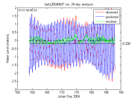
The first example is from Ballyheige, a town at the entrance to the Shannon River in western Ireland (bally20040607.xls). To get a feel for the use of the features described above, the reader can run a 30-day analysis of input file bally20040607.xls which contains water levels sampled at 5-minute intervals at Ballyheige (Data supplied courtesy of the Irish Geological Survey, Dublin, Ireland). After selecting this file the data box will display the number of days in the file followed by the date and time of the first record and the file name. After it has turned green, press the ANALYZE button to begin the analysis.

A window graph will appear displaying the observed water level (red), the astronomic tide (blue) and the residual (green) or difference between observed and predicted.. A pop-up message should also appear indicating a data gap within the file (8,340 records found, 8,353 expected). Whenever this message is seen, the cause should be sought by examining the input file. The gap in this example is too small to be seen in the 30-day plot. Using the 3-day plot feature, the gap can be clearly seen mid-morning on Julian day 173 (21-Jun-2004) at the point where the red curve abruptly shifts to the right by one hour. This is a time shift rather than a simple data gap and it means that all of the times past this point must be reduced by one hour. To skip the correction and proceed with the analysis, open the Excel file and move the worksheet labeled ’Fixed_file’ to the first position in the example workbook.

Figure 3. High Band Periodogram.

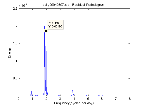
After loading and reading the fixed file, run the analysis again with the high band periodogram turned on. A Fourier periodogram will appear displaying two prominent peaks at adjacent frequencies. Using the data cursor, click on the left peak. An x-axis reading of approximately 1.862 cpd should be visible. Clicking on the peak to the right, 1.966 cpd should appear (Figure 3). The first frequency falls midway between constituents 2N2 and MU2; The second midway between LAM2 and L2. For the first stage of analysis with the five major constituents, the RMS error will read ±0.138 m and the percent reduction in variance (%R_Var) should read 98.15.

Tidal harmonic analysis is a form of multivariate analysis. To monitor the variables (constituent amplitude and phase) employed in a step-wise (stage) analysis the user should consider entering the amplitude and phase of all the constituents involved at each stage on a separate worksheet. One has already been entered in the bally20040607.xls file (tab labeled Stage Analysis). Selecting all four constituents 2N2, MU2, LAM2, and L2 produces a large change in the tidal amplitudes indicating that this choice is unacceptable for a series of this length. Choosing the one constituent near each peak with the greatest amplitude will produce a better result. After selecting MU2 and LAM2, the RMS error is reduced to ±0.109 m and %R_Var is increased to 98.80 percent.

In the next stage of the analysis, the first dominant peak suggests constituents Q1 and RHO1 and the second one matches the quarter-diurnal constituent, M4. Referring again to the Stage Analysis worksheet, RHO1 and M4 emerge as the most reasonable choices, reducing the RMS error to ±0.105 m and increasing %R_Var to 98.88 percent. In the final stage, MNS2, K2, M3, MN4, MS4 and M6 are added, reducing RMS error to ±0.100 m and increasing %R_Var to 98.98 percent. Noting the change in amplitude and phase for S2 at this stage may be surprising to some users, but in this instance it is clearly linked to relatively large amplitude in the luni-solar semidiurnal constituent, K2. K2 is often one of the major constituents in regions where the tide type is fully semidiurnal and the range is more than two meters (the mean range at Ballyheige is approximately three meters). Normally the K2 spectral peak is not pronounced in a short series because of its proximity to S2 which is included at the outset as one of the major constituents.

During the course of the above four stages, the peak energy shown in the periodogram falls by two orders of magnitude – from about 2 x 10^-3 to about 3 x 10^-5 m²/cpd. At this point we may enter a name and save the 15 constituents selected in a tidal constants file (e.g., Ballyheige_MSL to indicate that no offset from MSL was used).

Chesapeake Bay, USA

The second example is from a water level station at the Chesapeake Bay entrance (cbbt20021101.xls) courtesy of the U.S. National Oceanic and Atmospheric Administration (NOAA). This example also involves a 30-day analysis of water levels. The file named cbbt20021101.xls was obtained from the NOAA Tides & Currents web site and includes hourly water level data for 30 days beginning November 1, 2002. As with the previous example, a stage analysis for this file can be found on a separate worksheet in the Excel workbook. Tidal type here is mixed, mainly semidiurnal.

Analysis in stages yields 13 constituents for this file (Q1, O1, M1, K1, J1, OO1, MNS2, MU2, N2, M2, L2, S2 and K2) but, unlike example 1, the resulting model accounts for only 71.33 percent of the variance in water level. The reason why can be clearly seen in the residual curve for the window plot of the 30-day series. During this particular month, a subtidal oscillation was present at the bay entrance whose amplitude at times exceeded the amplitude of the astronomical tide. Switching to the low band periodogram, a peak frequency is shown at 0.2069 cpd (period = 4.83 days). Although a longer analysis would improve estimates of harmonic constituents such as S2 and K2 in the astronomical tide model, the increase in %R_Var would be small compared to the subtidal energy.

Special Features

Figure 4. Water level history for Hampton Roads, VA, September, 2003.

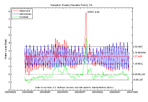
Providing tidal constants for water level predictions is one application of TAPtides. It is also useful for informative graphs displaying monthly water level histories at active monitoring stations. Water levels in near real time are now routinely displayed at NOAA PORTS stations on the web. These contain plots typically covering the past three days showing whether observed water levels are trending above or below predicted levels. A monthly plot can add value to this product by displaying monthly and weekly variations in tidal range in relation to non-tidal events such as a transient storm surge appearing in the residual curve. An example of a monthly plot is shown in Figure 4, at the Hamptons Roads, VA water level station during Hurricane Isabel. The observed water levels are shown in red, the fitted astronomical tides in blue, and the residuals containing the storm surge component in green. These figures are useful in understanding the extreme storm tides that result from the superposition of storm surge and astronomical tides.

Tidal Predictions

Figure 5. TAPtides prediction page.

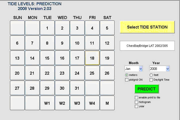
The TAPS window for performing tidal harmonic predictions of water levels may be opened from the SMS interface by clicking on the Data menu and then selecting Tidal Predictions | Water Levels. The window will display a list box in the upper right corner with the names of tidal constituent files created from previous Tidal Harmomic Analysis. As examples, two MATLAB data files (extension .mat) should appear from the Ballyheige and Chesapeake Bay analyses described in the previous section. Double click on either one to start.

After double clicking on a file, the file name and analysis date (year and Julian day starting) is displayed in the data box. Set the month and year of the required predictions along with the units desired (these units are independent of the units used in TAPtides analysis). Check boxes are available to turn on a plot grid and allow a change from Local Standard Time (LST) to Local Daylight Time (LDT) always assuming that LST was used during analysis. Pressing the large PREDICT button will then populate the calendar matrix at left with the days of the month and year selected. A daily, weekly or monthly plot of the predicted tide is displayed after pressing the appropriate button.

Printing to a file

The enable print to file check box below the PREDICT button allows the user to print 12-minute tidal height predictions to a text file for the month and year selected. If the year box is also checked, predictions are printed for the year selected using a 30-minute prediction interval. Excel calendar date and time is printed for each height value.

Histogram (Percentiles)

Figure 6. TAPtides height-frequency histogram for Ballyheige, Ireland.

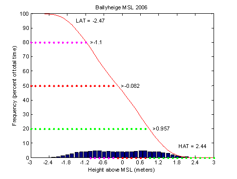
To display a histogram of predicted tidal heights as a percentage of total time, check the histogram box before pressing the PREDICT button. A cumulative curve will appear with percentile markings for the heights that are equaled or exceeded 20, 50 and 80 percent of the time for the month selected. If the year box is also checked, the percentages refer to total time for the year selected.

LAT and HAT estimates

If the tidal constants file selected does not contain a vertical datum offset (i.e., MSL-LAT=0.0), the histogram of predicted tidal heights will display the lowest astronomical tide (LAT) and the highest astronomical tide (HAT) for the month or year selected (Figure 6). Final estimates of LAT and HAT for use as reference datums can be found using the Analysis program (see Vertical Datums).

HAT estimate

If the tidal constants file selected does contain a vertical datum offset (i.e., MSL-LAT>0.0), the histogram of predicted tidal heights will reference heights above LAT and display the highest astronomical tide (HAT) for the month or year selected. Although generating most tidal height predictions relative to HAT would be confusing due to largely negative numbers, HAT is a good vertical reference for comparing storm tide peaks. HAT marks the extreme upper limit of the astronomical tide for a given time and place and its contour against the shore is often visibly marked (e.g., algal lines on rocks and piles). Normal tides will reach this contour in most, but not all years. And by using HAT as a reference, one can compare "extratidal" water levels between locations that have different tidal ranges.

Analyzing Storm Surge and Storm Tides

Figure 7. Storm tide and storm surge at Yorktown, VA, Tropical depression ERNESTO, 1-Sep-2006.

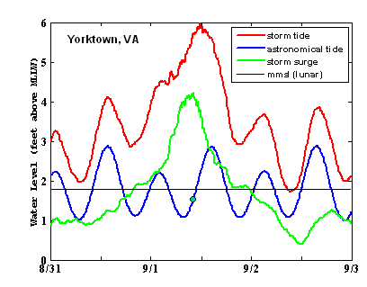
Storm tides are water levels made higher by the superposing of astronomical tides with storm surge, the transient change in water level resulting from the effects of a storm. In the United States, the term ’storm surge’ is used most often in connection with hurricanes and tropical storms, although tropical depressions and extra tropical storms or ’northeasters’ produce damaging storm surge as well. TAPtides is uniquely suited for conducting post-storm investigations of storm surge – it readily performs the task of separating the storm surge from water level observations and shows the nature of its interaction with the astronomical tide to produce the resulting water level extremes. An example from a NOAA tide station at Yorktown, Virginia, is shown in Figure 7. It was created from a TAPtides 29-day analysis of Yorktown records following a visit by tropical depression ERNESTO on 1 September, 2006.

Figure 7 provides a good illustration of the importance of ’timing’ between the arrival of the storm surge peak and the stage of the astronomical tide. The peak storm surge occurred much closer to low tide than high tide at Yorktown on the morning of September 1. The storm surge occurred during tropic tides evidenced by a strong diurnal inequality in the daily highs (Figure 7). The tides are mixed, mainly semidiurnal in this area. Thus the risk of an exceptional high storm tide was by no means spread evenly over a 24-hr period given the possibility of the storm surge peak arriving at another time. Figure 7 demonstrates the utility of the MATLAB figure editor in changing features such as scaling and labeling of figure axes, figure legends, and line thickness

Additional Information

Questions about this CHETN can be addressed Alex Sánchez at (601-634-2027), FAX (601-634-3433), or e-mail: [mailto: Alejandro.Sanchez@usace.army.mil Alejandro.Sanchez@usace.army.mil]. This Technical Note should be referenced as follows:

References

• Bloomfield, P. (2000). "Fourier Analysis of Time Series: An Introduction." John Wiley & Sons, New York, 258 pp.

• Boon, J. D. (2004, 2007). "Secrets of the Tide: Tide and Tidal Current analysis and Predictions, Storm surges and Sea Level Trends." Horwood Publishing, Chichester, U.K. 212 pp.

• Cartwright, D. E. (2000). "Tides: A scientific history." Cambridge University Press, 292 pp.

• Doodson, A. T., and Warburg, H. D. (1944). "Admiralty Manual of Tides." Admiralty Charts and Publications, London, England, 270 pp.

• Munk, W. H. and Cartwright, D. E. (1966). "Tidal Spectroscopy and Prediction." Phil. Trans. Royal Society of London. Series A, Mathematical and Physical Sciences, Vol. 259, No. 1105, pp. 533-581.

• Pugh, D. T. (2004). "Changing Sea Levels: Effects of Tides, Weather and Climate." Cambridge University Press, 265 pp.

• Schureman, P. (1958). "Manual of Harmonic Analysis and Prediction of Tides." U.S. Dept of Commerce, Coast and Geodetic Survey. Special Publication No. 98, Washington, D.C., 317 pp.

---

CMS Utilities