Flow over a bump: Difference between revisions
Jump to navigation
Jump to search
| Line 4: | Line 4: | ||
== Setup == | == Setup == | ||
The spatial domain consists of a rectangular | The spatial domain consists of a rectangular | ||
{{Equation| <math> z_b = \begin{ | {{Equation| <math> z_b = \begin{cases} | ||
0 \forall x<8m \\ | |||
0.2-0.05(x-10)^2 \forall 8 \leq x \leq 12 \\ | |||
0 \forall x>12 | |||
\end{cases} | |||
</math> |2=1}} | |||
where <math>\eta</math> is the water surface elevation, <math>\rho</math> is the water density, <math>\rho_a</math> is the air density, <math>g</math> is the gravitational acceleration, <math>W</math> is the wind speed, <math>h</math> is the water depth, and <math>C</math> is a constant of integration. | where <math>\eta</math> is the water surface elevation, <math>\rho</math> is the water density, <math>\rho_a</math> is the air density, <math>g</math> is the gravitational acceleration, <math>W</math> is the wind speed, <math>h</math> is the water depth, and <math>C</math> is a constant of integration. | ||
Revision as of 23:09, 14 December 2010
UNDER CONSTRUCTION
Setup
The spatial domain consists of a rectangular
| (1) |
where is the water surface elevation, is the water density, is the air density, is the gravitational acceleration, is the wind speed, is the water depth, and is a constant of integration.
Model Setup
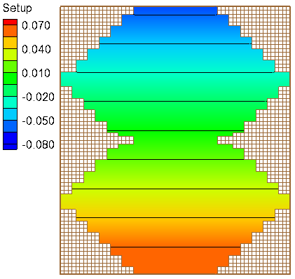
A computational grid with constant water depth of 5 m and irregular boundaries is used in order to test the model performance. The computational grid has 60 columns and 70 rows and a constant resolution of 500 m.
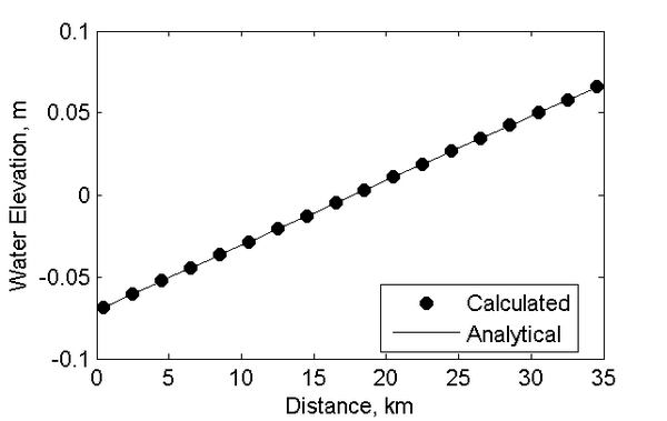
Results

