Hot Start

The term Hot start refers to starting a simulation with an initial condition other zero (cold start). Hot starts are used for specifying initial conditions or restarting simulations at intermediate times. The hot start controls are set in the Flow tab of the CMS-Flow Model Control window.

Hot Start File

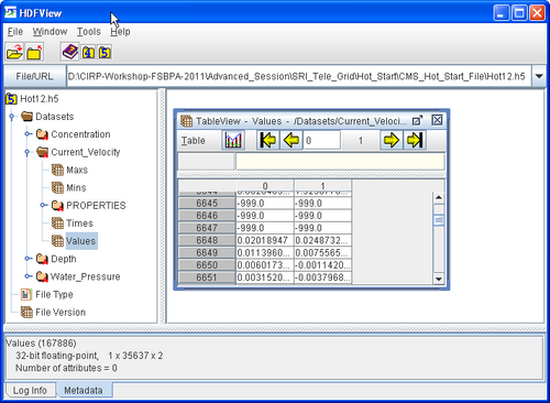
Figure 2. XMDFView showing the structure of the CMS Hot Start File.

The CMS hot start feature CMS lets the user restart simulations that have been stopped due to electric outages, hardware malfunctions, or model crashes. In the case of a model crash the user, may restart the model using larger solver iterations and/or time steps to stabilize the simulation. The user has the option to specify a hot start output time or an interval for outputting a recurring hot start file. Every time the hot start file is written, it overwrites the previous information. The CMS Hot Start file saves information on the water elevation (pressure), and current velocities. If the sediment transport is active, then the water depth, and sediment concentrations are also saved for each size class. The CMS hot start file is a binary XMDF file, has the name Hot_Start.h5 and is saved in the directory of the CMS-Flow files. Figure 1 shows the structure of the hot start file. After saving a CMS Hot Start file, it is a good idea to rename the file with a different name before using it as an initial conditions file. This way, the file will not be overwritten in future simulations.

Table 1. Hot Start CMS-Flow Cards

Card	Arguments	Default	Range	Description
HOT_START_OUTPUT_FILE	CHARACTER	none	none	Julian hour.
HOT_START_TIME	REAL	none	none	Sets the hot start output time.
AUTO_HOT_START_INTERVAL	REAL	none	none	Sets the recurring hot start output time.

Initial Conditions File

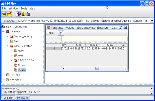
Figure 3. Dataset Toolbox showing a time step sample of the water elevation and current velocity datasets for use in a hot start (initial condition) file.

There are several situations where it is convenient to specify a user defined hot start file. For example, if the user forgets to setup the model output a hot start file or when running steady state conditions. A hot start file can easily be created and exported by the user from the SMS interface. The model requires at water levels, current velocities, concentrations, and water depths. Any datasets that are missing from the initial file. It is important to note that the names and paths of the initial condition datasets is important.

Table 2. Path and name for initial condition file variables.

Variable	Path and Name
Water surface elevation	Datasets\Water_Elevation
Current velocity	Datasets\Current_Velocity
Sediment concentrations	Datasets\Concentration
Salinity concentrations	Datasets\Salinity

The steps for creating a user defined hot start or initial condition file from a CMS-Flow solution file are outlined below.

Import CMS-Flow grid and solution file.
Sample a time step of the solution datasets for use in the initial condition
1. Click on Data | Data Calculator
  1. Under the Tools section, select Sample time steps.
  2. Under the Datasets section, click on the Water Elevation
Export the initial condition datasets to an XMDF file

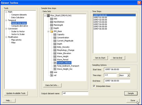
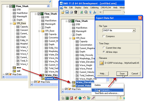
Figure 3. Dataset Toolbox showing a time step sample of the water elevation and current velocity datasets for use in a hot start (initial condition) file.

Figure 4. Dataset Toolbox showing a time step sample of the water elevation and current velocity datasets for use in a hot start (initial condition) file.

Table 3. CMS-Flow card for specifying the initial condition file.

Card	Arguments	Default	Range	Description
INITIAL_STARTUP_FILE	CHARACTER	none	none	Julian data in YYDDD with YY being last two digits of the year, and DDD the Julian day of the year.

Global Output

Figure 1. Output tab in SMS 11.0

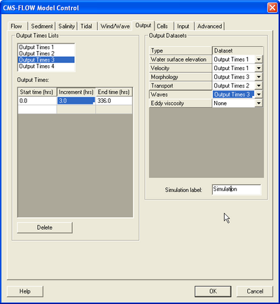
Global output refers to the variables that are output on every active cell on the grid. The global output options are specified in Output tab of the CMS-Flow Model Control window. More information on the global output variables, groups and CMS-Flow cards is provided in the sections below.

Output Datasets

A description of the CMS-Flow cards used to specify the global output variable datasets is provided below.

Table 1. Advanced output datasets.

Output Dataset	Group	Description	Units
Current_Velocity	Velocity	Depth-averaged and cell-centered current velocity vector dataset and with respect to local grid coordinates	m/s
Current_Magnitude	Velocity	Depth-averaged and cell-centered current velocity magnitude dataset	m/s
Water_Elevation	Water surface elevaation	Cell-centered water surface elevation	m
Eddy_Viscosity	Eddy viscosity	Cell-centered horizontal eddy viscosity	m^2/s
Concentration	Transport	epth-averaged and cell-centered sediment concentration	kg/m^3
Capacity	Transport	Depth-averaged and cell-centered sediment concentration capacity	kg/m^3
Total_Sediment_Transport	Transport	Depth-averaged and cell-centered total-load sediment transport	m^2/s
Salinity	Transport	Depth-averaged and cell-centered sediment concentration capacity	kg/m^3
Depth	Morphology	Cell-centered still water depth	m
Morphology_Change	Morphology	Cell-centered morphology (bed) change. Positive is accretion and negative is erosion	m
Wave_Height	Waves	Cell-centered significant wave height	m
Wave_Height_Vec	Waves	Cell-centered significant wave height vector	m
Wave_Period	Waves	Cell-centered peak wave period	s

Table 2. Output datasets and groups

Card	Arguments	Default value	Description
WSE_OUT_TIMES_LIST	INTEGER	0	Output time series id for the water surface elevation in m.
VEL_OUT_TIMES_LIST	INTEGER	0	Output time series id for currentvelocity and magnitude in m/s.
MORPH_OUT_TIMES_LIST	INTEGER	0	Output time series id for the water depth and morphology (bed) change in m.
TRANS_OUT_TIMES_LIST	INTEGER	0	Output time series id for sediment transport rates, concentations, and salinity.
WAVES_OUT_TIMES_LIST	INTEGER	0	Output time series id for the wave height in m, period in sec, and wave vectors.
EDDY_VISCOSITY_OUT_TIMES_LIST	INTEGER	0	Output time series id for the eddy viscosity in m^2/s.
VISC_OUT_TIMES_LIST	INTEGER	0	Output time series id for the eddy viscosity in m^2/s.
WIND_OUT_TIMES_LIST	INTEGER	0	Output time series id for wind velocity and magnitude in m/s.
STRESS_OUT_TIMES_LIST	INTEGER	0	Output time series id for mean bed shear stress in Pa.
WAVE_OUTPUT_DETAILS	ON \| OFF	OFF	Outputs additional wave variables including wave direction, radiation stresses, breaking dissipation and roller energy.

Output Time Series and Lists

The times at which each group is output is determined by the selecting one of four user defined output time series or lists. In SMS versions 10.1 and earlier, the output time series were used. However, because the output time series can become very large for long-term simulations, the time series have been replaced by lists in which the output times are specifying a list of starting, ending and increments. This option is more compact and also makes it easier to manually change the output options in the cmcards file.

Table 3. Advanced output datasets.

Card	Aguments/Format	Description
TIME_SERIES_1	[length of list 1] [output times for list 1]	Output time series for list 1 in hours.
TIME_SERIES_2	[length of list 2] [output times for list 2]	Output time series for list 2 in hours.
TIME_SERIES_3	[length of list 3] [output times for list 3]	Output time series for list 3 in hours.
TIME_SERIES_4	[length of list 4] [output times for list 4]	Output time series for list 4 in hours.
TIME_LIST_1	[number of sublists] [sublist 1: start, end, increment] [sublist 2: start, end, increment]...	Sublist(s) for output time series 1. For each sublist, the arguments are starting time, end time and increment in hours.
TIME_LIST_2	[number of sublist] [sublist 1: start, end, increment] [sublist 2: start, end, increment]...	Sublist(s) for output time series 2. For each sublist, the arguments are starting time, end time and increment in hours.
TIME_LIST_3	[number of sublist] [sublist 1: start, end, increment] [sublist 2: start, end, increment]...	Sublist(s) for output time series 3. For each sublist, the arguments are starting time, end time and increment in hours.
TIME_LIST_4	[number of sublist] [sublist 1: start, end, increment] [sublist 2: start, end, increment]...	Sublist(s) for output time series 4. For each sublist, the arguments are starting time, end time and increment in hours..

XMDF Output

The default option in CMS is to output all output groups to the same XMDF file (*_sol.h5). This option works well as long as the solution does not get too big. If the solution becomes too big, the SMS interface may have trouble reading the file. The option is also avaible to output different variable groups into separate XMDF files which helps reduce the file and makes it easier to visualize individual datasets in SMS. This feature is available in CMS-Flow Versions 4, Release 5 and more recent. This is done by either manually modifying the cards in the Output section of the cmcards file or by using new Advanced Cards. A list of the cards and their description is provided in the table below.

Table 2. XMDF file .

Card	Argument Type	Format	Example	Default	Version
WSE_OUT_FILE	CHARACTER	[<file path>/<file name>]	"<simulation label>_wse.h5"	"<simulation label>_sol.h5"	V4R5
VEL_OUT_FILE	CHARACTER	[<file path>/<file name>]	"<simulation label>_vel.h5"	"<simulation label>_sol.h5"	V4R5
VISC_OUT_FILE	CHARACTER	[<file path>/<file name>]	"<simulation label>_visc.h5"	"<simulation label>_sol.h5"	V4R5
TRANS_OUT_FILE	CHARACTER	[<file path>/<file name>]	"<simulation label>_trans.h5"	"<simulation label>_sol.h5"	V4R5
MORPH_OUT_FILE	CHARACTER	[<file path>/<file name>]	"<simulation label>_morph.h5"	"<simulation label>_sol.h5"	V4R5
WAVES_OUT_FILE	CHARACTER	[<file path>/<file name>]	"<simulation label>_wave.h5"	"<simulation label>_sol.h5"	V4R5
GLOBAL_WATER_LEVEL_OUTPUT	CHARACTER CHARACTER	[<file path>/<file name>] [<dataset path>]	"<simulation label>_wse.h5"	"<simulation label>_sol.h5"	V4R5
GLOBAL_VELOCITY_OUTPUT	CHARACTER CHARACTER	[<file path>/<file name>] [<dataset path>]	"<simulation label>_vel.h5"	"<simulation label>_sol.h5"	V4R5
GLOBAL_MORPHOLOGY_OUTPUT	CHARACTER CHARACTER	[<file path>/<file name>] [<dataset path>]	"<simulation label>_morph.h5"	"<simulation label>_sol.h5"	V4R5
GLOBAL_TRANS_RATE_OUTPUT	CHARACTER CHARACTER	[<file path>/<file name>] [<dataset path>]	"<simulation label>_trans.h5"	"<simulation label>_sol.h5"	V4R5

Notes:

The dataset path is not used by the CMS-Flow and is therefore not necessary to include.
In CMS-Flow versions ealier than V4R5, the above output cards are not used and all of the variable groups are output to the same XMDF file (*_sol.h5).

XMDF File Compression

The standard CMS-Flow output is written to an XMDF file with the name <Case Name>_sol.h5. The binary file may be written in compressed format using the card described in the table below.

Table 4. CMS-Flow card for compressing the XMDF output file

Card	Arguments	Default value	Description
XMDF_COMPRESSION	ON \| OFF	OFF	Compresses the h5 file by a factor of about 7

ASCII Output

In addition to the XMDF output file, CMS-Flow provides the output two types of ASCII output files:

Tecplot snap shot (*.dat), and history files (*.his)
SMS Super ASCII files (*.sup, *.xy, *.dat)

The CMS-Flow cards used for outputting these two types of files are described in the Table below.

Table 3. CMS-Flow cards used to output Tecplot and SMS Super ASCII files.

Card	Arguments	Description	Default value
GLOBAL_TECPLOT_FILES	ON \| OFF	Outputs Tecplot ASCII files	OFF
GLOBAL_SUPER_FILES	ON \| OFF	Outputs Tecplot ASCII files	OFF

Output Cells

Figure 1. Cells tab in SMS 11.0

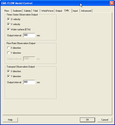
Time series at selected Obervation cells is set in the Cells tab of the CMS-Flow Model Control window. A description of CMS-Flow cards used for specifying Observational cells are described below.

Table 5. CMS-Flow card for compressing the XMDF output file

Card	Arguments	Description
TIME_SERIES_INCREMENT	REAL	Sets the output time increment for the Time series Observation points.
ELEV_OBS_CELLS_BEGIN	none	Marks the begging of an Times series Observation point list.
ELEV_OBS_CELLS_END	none	Marks the end of an Times series Observation point list.
FLOW_RATE_INCREMENT	REAL	Sets the output time increment for the Flow rate Observation points.
FLOW_OBS_CELLS_BEGIN	none	Marks the end of an Flow rate Observation point list.
FLOW_OBS_CELLS_END	none	Marks the end of an Flow rate Observation point list.
Q_TRANS_INCREMENT	REAL	Sets the output time increment for the Flow rate Observation points.
Q_TRANS_OBS_CELLS_BEGIN	none	Marks the end of an Transport Observation point list.
Q_TRANS_OBS_CELLS_BEGIN	none	Marks the end of an Transport Observation point list.

Statistics

CMS V4.0 has the option to calculate statistics over the whole model domain for a user-specified time period. This option is accessed using the advanced cardss. The starting time, end time, and time interval should be specified in hours with respect to the model start time. The time interval should be larger or equal to the hydrodynamic time step. When activated the global statistics will be output in the same solution file within a subfolder named stats.

This option outputs the statistics for hydrodynamics, sediment and salinity transport. If only the statistics for one group

Hydrodynamics:

Maximum current velocity
Maximum water level
Residual currents (vectors and magnitude)
Hydroperiod
Maximum spatial gradient for water levels
Maximum spatial gradient for current magnitude

Sediment Transport and Morphology Change:

Maximum total load transport rate, m^2/hr
Net total load sediment transport rates, m^2/hr
Average total load sediment transport rates, m^2/hr
Gross total load sediment transport rates, m^2/hr
Positive and negative total load transport rates (in x and y directions), m^2/hr
Maximum spatial gradient of bathymetry

Salinity Statistics:

Mean Salinity

Table 6. CMS-Flow cards related to output statistics

Card	Arguments	Description	Default value
GLOBAL_STATISTICS	[t0] [tn] [dt]	Calculates global statistics if specified	none
FLOW_STATISTICS	[t0] [tn] [dt]	Calculates flow statistics if specified	none
SEDIMENT_STATISTICS	[t0] [tn] [dt]	Calculates sediment statistics if specified	none
SALINITY_STATISTICS	[t0] [tn] [dt]	Calculates salinity statistics if specified	none

Numerical Methods

Solution Scheme

This refers to the temporal discritization of the hydrodynamic, sediment and salinity transport equations. There are two options in CMS: 1. Implicit - First order backward Euler scheme. Uses a time step on the order of 5-15 minutes. Appropriate for cases which can be simulated with large computational time steps such as long term morphology change at inlets. 2. Explicit - First order forward Euler scheme. Uses a time step on the order of 0.5-1.0 second. Appropriate for cases that vary quickly in time such as flooding or barrier island breaching.

Card	Arguments	Default	Range	Description
SOLUTION_SCHEME	CHARACTER	EXPLICIT	EXPLICIT \| IMPLICIT	Determines the solution scheme used in CMS-Flow.

Solver Options

The four different solvers implemented in the implicit solution scheme are the Gauss-Seidel, Gauss-Seidel with Successive-Over-Relaxation, BICGSTAB, and GMRES. The same solver is applied to flow, sediment and salinity. The default solver is the GMRES. The solver may be changed using the advanced card in the table below.

Card	Arguments	Default	Range	Description
MATRIX_SOLVER	CHARACTER	GMRES	GAUSS-SEIDEL \| GAUSS-SEIDEL-SOR \| BICGSTAB \| GMRES	Selects the matrix solver for flow, sediment and salinity.
HYDRO_MAX_ITERATIONS	INTEGER	Function of grid size	>0	Sets the maximum number of iterations for the flow (hydro) solver (outer loop). Typical range: 30-50 for GAUSS-SEIDEL and GAUSS-SEIDEL-SOR, and 20-30 for BICGSTAB and GMRES.
PRESSURE_ITERATIONS	INTEGER	Depends on Solver	>0	Sets the number of solver iterations for the pressure equation (inner loop). Typical range: 80-100 for GAUSS-SEIDEL and GAUSS-SEIDEL-SOR, and 15-25 for BICGSTAB and GMRES.
VELOCITY_ITERATIONS	INTEGER	Depends on Solver	>0	Sets the number of solver iterations for the velocity or momentum equations (inner loop). Typical range: 20-30 for GAUSS-SEIDEL and GAUSS-SEIDEL-SOR, and 5-10 for BICGSTAB and GMRES.
SEDIMENT_MAX_ITERATIONS	integer	20	>0	Maximum number of iterations (outer loop) for the sediment transport
SALINITY_MAX_ITERATIONS	integer	20	>0	Maximum number of iterations (outer loop) for the salinity transport

Advection scheme

As in the case of the implicit solution scheme, the same advection scheme is applied for the flow, sediment and salinity transport equations. There are three choices for advection schemes with upwinding in the implicit model: hybrid, exponential and HLPA. The hybrid scheme is fast but is the most diffusive. The exponential scheme is based on the 1D analytical solution to an advection-diffusion equation and produces very stable results. The HLPA is very stable and non-diffusive, but requires slightly more computational time. For most applications, the exponential scheme is recommended and is set as the default. The advection scheme may be change using the advanced card

Table 5. CMS-Flow cards related to numerical methods.

Card	Arguments	Default	Range	Description
ADVECTION_SCHEME	CHARACTER	EXPONENTIAL	NONE \| HYBRID \| EXPONENTIAL \| HLPA	Sets the advection scheme for flow, sediment and salinity.

Wetting and Drying

Table 5. CMS-Flow cards related to numerical methods.

DRYING_DEPTH	REAL	Calculated based on solution scheme and courant number	none	Sets to the time step for hydrodynamics in seconds.
WATER_PONDING	CHARACTER	OFF	ON \| OFF	Turns On or Off water ponding. If water ponding is Off, isolated bodies of water will become dry.
ONE_CELL_WIDE_CHANNELS	CHARACTER	ON	ON \| OFF	Limits wetting and drying to areas with at least 3 cells wide. When turned off, the model stability is improved.

Parallelization with OpenMP

Both Intel and AMD processors now are shipping chips with multiple cores/processors (henceforth referred to as "processors") available. CMS-Flow is now configured to make use of these extra processes that are available on newer machines.

Additional information on using Multiple Processors with CMS-Flow can be found here.

Table 5. CMS-Flow cards related to numerical methods.

Card	Arguments	Default	Range	Description
NUM_THREADS	INTEGER	1	Determines the number of threads used for parallel processing.
OPENMP_THREADS	INTEGER	1	Determines the number of threads used for parallel processing.

Scripting

Scipting refers to the automation of running multiple CMS runs with different parameters, without manually having to create and edit each alternative. The scripting process can include the following steps:

Setting up alternatives
Creating batch file
Plotting and analyzing results

Scripting can be done using a variety of software programs. The examples shown here were written in Matlab becase it is widely used, easy to read and convenient for plotting and analyzing results.

Setting Up Alternatives

‎

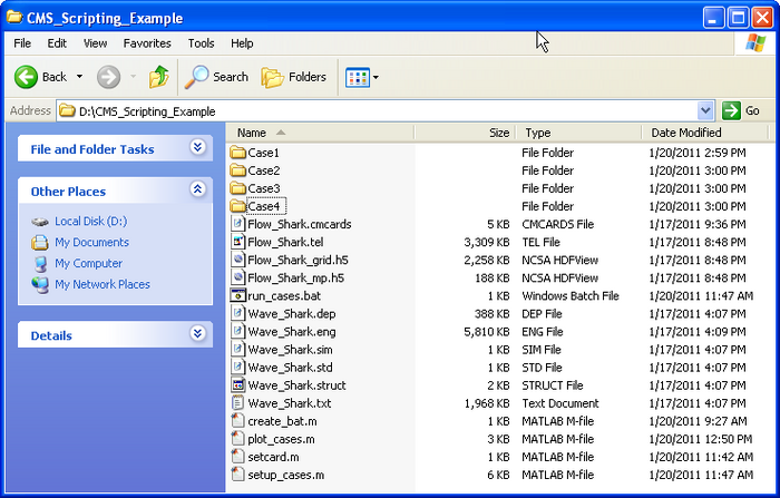
Figure 1. Example of scripting showing the files used.

In this example, 4 cases or alterantives are setup using the Matlab script below. The script copies the base setup files into subfolders and then modifies specific CMS-Flow cards in the *.cmcards file. The settings for each case are setup using a structure variable with field names corresponding to each CMS-Flow card (e.g. TIME_SERIES_INCREMENT). Separating each case into its own subfolder keeps the input and output separate and also allows for the different cases to be run at the same time.

% Matlab Script: setup_cases.m
clear all
flow = 'Flow_Shark';
wave = 'Wave_Shark';
ncases = 4; %Number of cases or alternatives  
r(1).MANNINGS_N_DATASET = '"Manning_Alt1.h5" "Flow_Shark/Datasets/ManningsN"';
r(1).WAVE_CURRENT_MEAN_STRESS = 'W09';
r(1).TIME_SERIES_INCREMENT = 1800;
r(2).MANNINGS_N_DATASET = '"Manning_Alt1.h5" "Flow_Shark/Datasets/ManningsN"';
r(2).WAVE_CURRENT_MEAN_STRESS = 'DATA2';
r(2).TIME_SERIES_INCREMENT = 900;
r(3).MANNINGS_N_DATASET = '"Manning_Alt2.h5" "Flow_Shark/Datasets/ManningsN"';
r(3).WAVE_CURRENT_MEAN_STRESS = 'W09';
r(3).TIME_SERIES_INCREMENT = 900;
r(4).MANNINGS_N_DATASET = '"Manning_Alt2.h5" "Flow_Shark/Datasets/ManningsN"';
r(4).WAVE_CURRENT_MEAN_STRESS = 'DATA2';
r(4).TIME_SERIES_INCREMENT = 600;
for i=1:ncases
  d = ['Case',int2str(i)];
  if ~exist(d,'dir')
    mkdir(d)
  end
  copyfile([wave,'.*'],d)
  copyfile([flow,'.*'],d)
  copyfile([flow,'_mp.h5'],d);
  copyfile([flow,'_grid.h5'],d)
  cards = fieldnames(r(i));
  file = ['.\',d,'\',flow,'.cmcards'];
  fork=1:length(cards)
    setcard(file,cards{k},r(i).(cards{k})); 
  end
end
return

The script above requires the subroutine below.

function setcard(cmcardsfile,card,value)
% setcard(file,card,value)
% Overwrites or appends a CMS-Flow card
% in the *.cmcards file
copyfile(cmcardsfile,'temp')
fid=fopen('temp','r');
fid2=fopen(cmcardsfile,'w');
nc=length(card);
ok = false(1);
if ~ischar(value)    
  value = num2str(value);
end
while 1    
  tline = fgets(fid);        
  if ~ischar(tline), break, end    
  if strncmp(card,tline,nc)        
    fprintf(fid2,'%s       %s %s' ,card,value,tline(end));                
    ok = true(1);        
    continue    
  end    
  nline = length(tline);    
  if (~ok && strcmp(tline(1:min(nline,14)),'END_PARAMETERS'))        
    fprintf(fid2,'%s       %s %s',card,value,tline(end));        
    fprintf(fid2,'%s' ,tline);        
    break 
  end    
  fprintf(fid2,'%s' ,tline);
end
fclose(fid);
fclose(fid2);
delete('temp')
return

Batch File

Although it is possible to launch CMS from Matlab a batch file is preferable to use a batch file because it allows running all of the cases without opening Matlab.

% Matlab Script: create_bat.m
cmsexe = 'cms2d_v4b42_x64p.exe'; %CMS-Flow executable
batfile = 'run_cases.bat'; %Output batch file
fid = fopen(batfile,'w');
for i=1:ncases 
  cmcards = ['.\Case',int2str(i),'\',flow,'.cmcards']; %CMS-Flow cmcards file
  fprintf(fid,'START %s %s %s',cmsexe,cmcards,char(10)); 
end
fclose(fid);
return

The following text shows what the resulting batch file (*.bat) looks like

START cms2d_v4b42_x64p.exe .\Case1\Flow_Shark.cmcards
START cms2d_v4b42_x64p.exe .\Case2\Flow_Shark.cmcards
START cms2d_v4b42_x64p.exe .\Case3\Flow_Shark.cmcards
START cms2d_v4b42_x64p.exe .\Case4\Flow_Shark.cmcards

To run the batch file, simply double click on the file and each case will launch separately in its own MS-DOS window.

Plotting

The following example reads the Observation Point time series output file (*_eta.txt) and plots the 3rd

% Matlab Script: plot_cases.m
close all 
eta = cell(ncases,1); 
for  i=1:ncases    
  etafile = ['.\Case' ,int2str(i),'\',flow,'_eta.txt' ]; %Water elevation
  eta{i} = load(etafile);    
end
figure
hold on
for i=1:ncases    
  h = plot(eta{i}(:,1),eta{i}(:,3),'-');  %3 is the index is the observation point index
end
ylabel('Water elevation, m')
xlabel('Elapsed Time, hr')
return

Units of Measurement

Variable	Units	Symbol
Water Surface Elevation	meters	$m$
Current Velocity	meters per second	$m/sec$
Flow Rate	cubic meters per second	$m^{3}/sec$
Salinity Concentration	parts per thousand	$ppt$
Sediment Concentration	kilogram per meter cubed	$kg/m^{3}$
Sediment Transport	meter squared per second	$m^{2}/sec$
Bed Shear Stress	kilogram per meter per second squared	$Pa$

CMS-Flow

CMS-Flow:Features

Contents

Hot Start

Hot Start File

Initial Conditions File

Global Output

Output Datasets

Output Time Series and Lists

XMDF Output

XMDF File Compression

ASCII Output

Output Cells

Statistics

Numerical Methods

Solution Scheme

Solver Options

Advection scheme

Wetting and Drying

Parallelization with OpenMP

Scripting

Setting Up Alternatives

Batch File

Plotting

Units of Measurement

Navigation menu

CMS-Flow:Features

Hot Start

Hot Start File

Initial Conditions File

Global Output

Output Datasets

Output Time Series and Lists

XMDF Output

XMDF File Compression

ASCII Output

Output Cells

Statistics

Numerical Methods

Solution Scheme

Solver Options

Advection scheme

Wetting and Drying

Parallelization with OpenMP

Scripting

Setting Up Alternatives

Batch File

Plotting

Units of Measurement

Navigation menu

Search