CMS-Flow:Features

Global Forcing

There are two main types of global forcing available in CMS-Flow, wind and wave. Global forcing means that the forcing is applied on a cell-by-cell nature, rather than forcing along a boundary.

Wind Forcing

Wind Curve

SMS 10.1

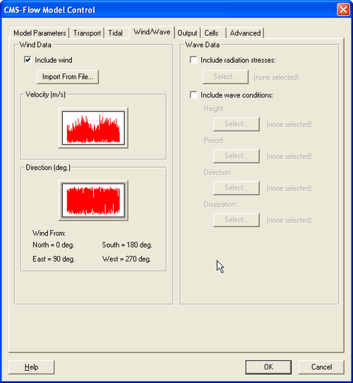
Temporally varying, spatially constant winds are input in CMS in the Wind Section of the CMS-Flow Model Control Window. To add wind forcing to a current CMS-Flow project click on CMS-Flow | Model Control and then on the Wind/Wave tab. Activate wind forcing by clicking on the Include Wind check box. Winds may be imported using an *.m2w file or by specifying a curve for wind speed and direction. To specify a curve for each click on the respective box which says Curve undefined which will open the XY Series Editor. The time series may be manually entered, copied or imported from an *.xys file in the XY Series Editor.

Spatially Variable Wind and Atmospheric Pressure CMS-Flow V4.0 and higher have the option to use spatially variable wind and atmospheric pressure forcing. Currently, this feature is specified in the advanced card section using the cards listed in the table below.

CMS-Flow cards related to wind

Card	Arguments	Type
WIND_OUT_TIMES_LIST	Id number of output times list	integer
WIND_DRAG_COEFFICIENT	kappa in Hsu (1988) (default 0.4)	real
WIND_INPUT_CURVE	Name of model parameter file followed wind curve path	character
ANEMOMETER_HEIGHT	Height of wind speeds	meter
OCEANWEATHER_WIND_FILE	Name of Oceanweather, Inc. wind file (*.win)	character
OCEANWEATHER_PRES_FILE	Name of Oceanweather, Inc. pressure file (*.pre)	character
OCEANWEATHER_XY_FILE	Name of Oceanweather, Inc. coordinate file (*.xy)	character
WIND_PRESSURE_FLEET_FILE	Name of fleet wind and pressure file	character
WIND_PRESSURE_GRID_PARAM	Nwlat,Nwlon,wLatMax,wLonMin,wLatInc,wLonInc	integer and real
WIND_PRESSURE_TIME_INCREMENT	wTimeInc	real

Wave Forcing

Temporally and spatially varying.

• Wave forcing is generally provided by the user selecting to use the Steering Module within SMS. The mapping of wave data from wave grid to flow grid is automated during the course of the steering process.
• If a choice is made not to use the steering process, the user must provide several datasets of information which has been mapped to the flow grid geometery.
  • Radiation stress gradient
  • Wave height
  • Wave period
  • Wave direction
  • Wave dissipation

CMS-Flow cards related to wave forcing (one-way coupling)

Card	Arguments	Type
WAVE_RSTRESS_DATASET	"File name" "Dataset path"	character
WAVE_HEIGHT_DATASET	"File name" "Dataset path"	character
WAVE_PERIOD_DATASET	"File name" "Dataset path"	character
WAVE_DIRECTION_DATASET	"File name" "Dataset path"	character
WAVE_DISSIPATION_DATASET	"File name" "Dataset path"	character

Salinity Transport

In many estuaries, the density gradients caused by spatial variations in salinity can be an important driving force in the circulation. Salinity is also a key water quality variable in estuaries, since it affects the chemical and biological processes. Salinity is simulated in the Coastal Modeling System (CMS) in a depth-averaged sense. This means that the estuary or body of water is assumed to be well mixed vertically and the salinity is constant over the water column.

The salinity transport equation is solved with an explicit, finite volume method. The advection term is discretized with upwind scheme, and the diffusion term is discretized with the standard central difference scheme.

The CMS-Flow salinity cards are listed in the table below.

Card	Arguments	Description	Versions
CALC_SALINITY	ON | OFF	Turns salinity on or off	>=v3.75
SALT_OUT_TIMES_LIST	integer	Index of times list of output times	>=v3.75
SALINITY_IC	real	Specifies the initial salinity value in ppt for the whole computational domain	>=v3.75
SALINITY_IC_ASCII	character	Specifies the file name of a scatter set file (*.pts) containing the coordiantes and initial salinity values to be interpolated using the Laplacian interpolation	>=4.0

Additional information on Salinity Transport in CMS-Flow can be found here.

Other Processes

Bottom Friction

SMS Project Explorer showing CMS-Flow project.

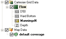
The bottom friction parameter (related to Manning $n$) is spatially varying (cell-specific) over the grid domain. The default value upon grid creation is 0.025. At times a user may desire to represent locations where added friction is needed due to structures or increased turbulence due to sharp changes in current speed. More information on using this feature of CMS-Flow can be found here.

Card	Arguments	Default	Range	Description	Versions
USE_WALL_FRICTION	CHARACTER	ON	ON | OFF	Turns on or off wall friction	>=3.5
MANNING_N_DATASET	CHARACTER CHARACTER	[<grid file>] [<grid name>//"Datasets/ManningsN"]	none	Grid file name and dataset path for the input Manning's n dataset	>=v3.5
MANNING_N_CONSTANT	real number	none	0.001-0.5	Specifies input Manning n dataset	>=v3.5
WAVE-CURRENT_MEAN_STRESS	character	W09	W09 | DATA2 | DATA13 | F85 | HT95	Defines the model used for calculating the mean bottom shear stress used in hydro	>=4.0

Hard Bottom

SMS Project Explorer showing Hard bottom dataset

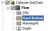
Hard Bottom is a morphologic constraint that provides the capability to simulate mixed bottom types within a single simulation. This cell-specific feature limits the erodibility of the constrained cells down to a specified depth below the water surface. More information on the use of hard bottom within the SMS can be found here.

CMS-Flow Model Control window showing the location where the hard bottom dataset is specified.

Variable D50

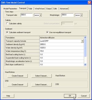
When sediment transport and morphology change are activated, sometimes it may be desired to designate areas of the grid to have a certain grain size. This cell-specific parameter allows each cell to take on the characteristics of a certain sediment grain size. More information on the use of variable grain size (D50) can be found here.

Eddy Viscosity

Eddy Viscosity in CMS-Flow is not a user definable parameter. A description of the advanced cards related to eddy viscosity is shown in the table below.

Card	Arguments	Default	Range	Description	Versions
TURBULENCE_MODEL	CHARACTER	SUBGRID	SUBGRID |FALCONER| PARABOLIC | MIXING-LENGTH	Specifies the turbulence model used	>=3.5
EDDY_VISCOSITY_CONSTANT	REAL	1.0E-6	>=1.0E-6	Constant contribution or base value of eddy viscosity	>=3.5
EDDY_VISCOSITY_BOTTOM	REAL	0.0667	0.01-0.2	Coefficient related to the contribution to eddy viscosity from the bottom shear	>=3.5
EDDY_VISCOSITY_HORIZONTAL	REAL	0.4	0.2-0.6	Coefficient related to the contribution to eddy viscosity from horizontal velocity gradients	>=3.5
EDDY_VISCOSITY_WAVE	REAL	0.5	0.2-1.0	Coefficient related to the wave bottom friction contribution to eddy viscosity	>=4.0
EDDY_VISCOSITY_BREAKING	REAL	0.05	0.04-0.08	Coefficient related to the wave breaking contribution to eddy viscosity	>=4.0

More information can be found here.

Other Features

Parallelization with OpenMP

Both Intel and AMD processors now are shipping chips with multiple cores/processors (henceforth referred to as "processors") available. CMS-Flow is now configured to make use of these extra processes that are available on newer machines.

Additional information on using Multiple Processors with CMS-Flow can be found here.

Advanced Output

The following advanced cards have been added to CMS v4.0 and higher for outputting additional output information, ASCII file output, and more.

Card	Arguments	Description	Default value
XMDF_COMPRESSION	ON | OFF	Compresses the h5 file by a factor of about 7	OFF
WAVE_OUT_TIMES_LIST	integer	Output time series id	0
EDDY_OUT_TIMES_LIST	integer	Output time series id	0
VISC_OUT_TIMES_LIST	integer	Output time series id	0
STRESS_OUT_TIMES_LIST	integer	Output time series id	0
BED_SHEAR_STRESS_OUT_TIMES_LIST	integer	Output time series id	0
GLOBAL_TECPLOT_FILES	ON | OFF	Outputs Tecplot ASCII files	OFF
GLOBAL_SUPER_FILES	ON | OFF	Outputs Tecplot ASCII files	OFF
GLOBAL_STATISTICS	[t0] [tn] [dt]	Calculates global statistics if specified	none
FLOW_STATISTICS	[t0] [tn] [dt]	Calculates flow statistics if specified	none
SEDIMENT_STATISTICS	[t0] [tn] [dt]	Calculates sediment statistics if specified	none
SALINITY_STATISTICS	[t0] [tn] [dt]	Calculates salinity statistics if specified	none

Matrix solver

The four different solvers implemented in the implicit model are the Gauss-Seidel, Gauss-Seidel with Successive-Over-Relaxation, BICGSTAB, and GMRES. The same solver is applied to flow, sediment and salinity. The default solver is the GMRES. The solver may be changed using the advanced card in the table below.

Card	Arguments	Description	Default value
SOLVER_TYPE	GAUSS-SEIDEL | GAUSS-SEIDEL-SOR | BICGSTAB | GMRES	Determines the numerical solver used	GMRES
HYDRO_MAX_ITER	integer	Maximum number of iterations (outer loop) for the hydrodynamics	20
SEDIMENT_MAX_ITER	integer	Maximum number of iterations (outer loop) for the sediment transport	20
SALINITY_MAX_ITER	integer	Maximum number of iterations (outer loop) for the salinity transport	20

Advection scheme

As in the case of the solver, the same advection scheme is applied for the flow, sediment and salinity transport equations. There are three choices for advection schemes with upwinding in the implicit model: hybrid, exponential and HLPA. The hybrid scheme is fast but is the most diffusive. The exponential scheme is based on the 1D analytical solution to an advection-diffusion equation and produces very stable results. The HLPA is very stable and non-diffusive, but requires slightly more computational time. For most applications, the exponential scheme is recommended and is set as the default. The advection scheme may be change using the advanced card

Card	Arguments	Description	Default value
ADVECTION_SCHEME	HYBRID | EXPONENTIAL | HLPA	Determines the advection scheme	EXPONENTIAL

Units of Measurement

Variable	Units	Symbol
Water Surface Elevation	meters	$m$
Current Velocity	meters per second	$m/sec$
Flow Rate	cubic meters per second	$m^{3}/sec$
Salinity Concentration	parts per thousand	$ppt$
Sediment Concentration	kilogram per meter cubed	$kg/m^{3}$
Sediment Transport	meter squared per second	$m^{2}/sec$
Bed Shear Stress	kilogram per meter per second squared	$Pa$

---

CMS-Flow