GenCade Example
This section includes step-by-step instruction of how to create and run a simple case in GenCade. A zip file is included at the end of this section, so the results can be reproduced on another computer. After completing this example, the user should be able to setup a simple GenCade grid, understand how the steps can be applied to a more complex case, run GenCade, and review results.
This simple case involves a straight shoreline (no regional contour), a groin, a beach fill, and an inlet. Variable grid resolution is not used.
Setup GenCade in the SMS
If this is the first time the GenCade interface has been used in the SMS on a specific computer, please follow the instructions in the GenCade User's Guide.
1. Open SMS 11.0 Development. Right click on Default Coverage under Map Data and scroll down to Type->Models->GenCade. Click Default Coverage again and notice the tools in the toolbar have changed.
2. Go to Edit->Projection. Under Horizontal, select Local Projection and change the units to U.S. Survey Feet. The vertical units should also be in U.S. Survey Feet. Click OK.
Draw Initial Shoreline, Grid, and Other Features
1. First, draw the grid frame. Click on Create 1-D Grid Frame in the toolbar. Draw a grid frame of any shape. Once the grid frame has been created, the line should turn purple. Click on Select 1-D Grid Frame. Double-click on the square at the center of the grid frame to open the Grid Frame Properties. Change the Origin X and Origin Y values to 0. Change the Angle to 180, and assign an I size of 10000 ft. Under I Cell Options, change the cell size to 50 ft. Click OK. Notice that the arrow next to the grid frame is pointed to the left on the computer screen. This means the water is below grid frame (if a person is walking along the grid frame, the water is to the left). Therefore, the initial shoreline should be drawn below the grid frame.
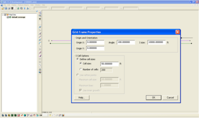
2. Click on Create Feature Arc to draw the initial shoreline. Draw the initial shoreline 200 ft below the grid frame. This can be done by using the measuring tool or looking at the x and y coordinates at the bottom of the screen. Make sure the initial shoreline extends past the grid frame. Click Select Feature Arc, double-click on the initial shoreline, and define the arc as Initial Shoreline.
Note: If the initial shoreline has already been created and is in x and y coordinates, it is very easy to drag the initial shoreline into GenCade. For this simple example, an initial shoreline (as a *.cst) can be created. Open Notepad or another text application on the computer. The first line should say COAST, and the second line should say 1. Since the initial shoreline will be a straight line, only two points are necessary. The third line should say 2 0. The first point is 100, -200 and the second point is -10100, -200. Save the file as a *.cst and drag into the SMS. Click Select Feature Arc, double-click on the initial shoreline, and define the arc as Initial Shoreline.
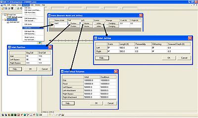
3. Select the Create Feature Arc button. Using the measuring tool, draw a 1000 ft arc at the center of the grid. Remember to draw the arc below the initial shoreline. Once the arc has been created, click on Select Feature Arc and double-click on the arc. Define the arc as an inlet and go to Attributes. Click on Volume. For this simple case, the initial and equilibrium volumes will be the same. See Figure 2 to see the input shoal volumes. Dredging will not be included in this example. Change Y Left and Y Right to 1.0. Make sure to name the inlet. If the inlet does not have a name, the inlet will be deleted.
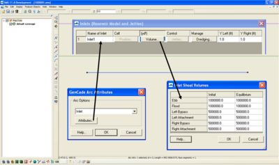
4. The inlet will be structured, so click on Create Feature Arc. Draw two lines perpendicular to the inlet. Make each arc 300 feet long (from the shoreline). Do not allow the lines to cross the inlet or the initial shoreline. Click on Select Feature Arc and define the arcs as Left Jetty on Inlet and Right Jetty on Inlet. Remember that on the computer screen, the left jetty will visually be on the right. Leave permeability as 0, select diffracting, and change the seaward depth to 6 ft for both jetties.
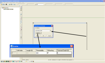
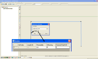
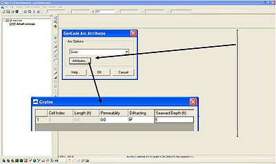
5. Click on Create Feature Arc to add the groin. Using the measuring tool, draw a 300 ft long groin (from the shoreline) at a distance of 2500 ft from the left extent of the grid. Again, make sure the end of the arc does not intersect the initial shoreline. This will result in the initial shoreline being divided into two separate sections which SMS cannot handle at this time. Double-click on the arc with the Select Feature Arc tool. Define the arc as a groin and click on Attributes. Keep the permeability at 0, check diffracting, and change the seaward depth to 6 ft.
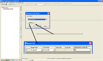
6. Draw the arc for the beach fill by selecting the Create Feature Arc tool. The beach fill will be 500 ft long, and begin at 3750 ft from the left extent and end at 4250 ft from the left extent of the grid. After selecting the feature arc, define the arc as a Beach Fill Event and go to Attributes. The Begin Date is 1 April 2009, the End Date is 1 June 2009, and the Added Berm Width is 50 ft.
Include Wave Gage
1. Select the Create Feature Point button. Draw the feature point for the wave gage at the center of the grid at any distance offshore.
2. Before defining the point as a wave gage, it is necessary to set up the wave information in Excel. Open Excel. The columns from left to right are the date, wave height, wave period, and direction. Right click on the first column and go to Format Cells. Under the Number tab, select Custom under Category. Type the format m/d/yyyy h:mm and click Ok. Type 1/1/2009 in the first cell. The output in the cell should be 1/1/2009 0:00. Include wave information for each hour for one year. The wave height is 0.5 m, the wave period is 6 seconds, and the direction is 10 degrees. Copy the columns and save the spreadsheet.
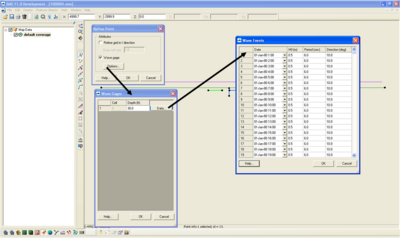
3. Return to the SMS. Click on the Select Feature Point button and double-click on the point representing the wave gage. Check wave gage under the Refine Point menu and click on Options. Assign a depth of 30 feet, and click on Data. Left click to highlight the first cell in the first column. Right click and scroll down to paste. It may take a minute or two to copy over the information. If any other task is performed on the computer while the wave information is being copied over, the SMS could freeze or crash. Click OK to exit the wave data menu. Now the wave gage point will have an arrow showing the direction of the wave for the first time in the series.
Convert to 1-D Grid
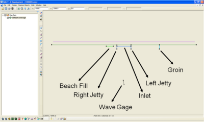
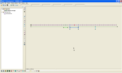
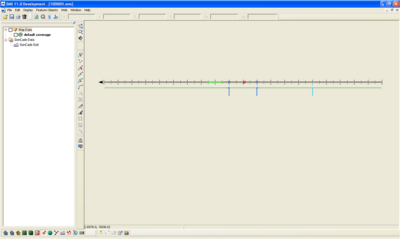
1. Right click on Default Coverage and scroll to Convert->Map->1D Grid. The Map->1D Grid will open. This window is identical to the Grid Frame Properties window. No changes need to be made to the grid, so click OK. The graphical window should look like Figure 9 below. Uncheck the default coverage to see only the GenCade grid.
Check Grid and Model Control
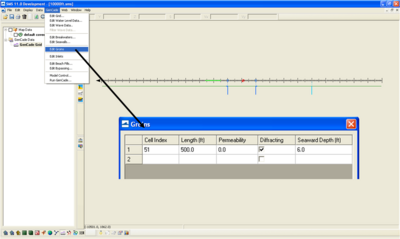
1. Go to the GenCade menu (between Data and Web) and go to Edit Groins. Verify the groin is in cell 51 and the length is 500 ft. Modify if necessary. The length is the distance from the grid to the end of the groin. In this case, the shoreline is 200 ft from the grid, so the groin is 300 ft.
2. Go to Edit Inlets in the GenCade menu. The inlet beginning cell should be 91 and the ending cell should be 110. Make the left and right bypass one cell wide (left bypass - cell 90 to 90; right bypass - cell 111 to 111). Click on Jetties. Ensure both the left and right jetties exist. The length of each should be 500 ft. The permeability and seaward depth should have been defined previously.
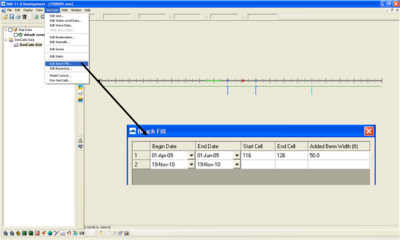
3. Go to Beach Fill. The Start Cell should be 116, and the End Cell should be 126. Double check the Begin Date, End Date, and the Added Berm Width.
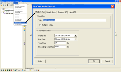
4. Go to Model Control in the GenCade menu. The first tab is Model Setup. The simulation title does not need to be changed. Under Computation Time, change the Start Date to 1-Jan-09 12:00 AM and the End Date to 1-Jan-10 12:00 AM. Change the Time Step to 0.5 hour and keep the Recording Time Step as the default (168 hours).
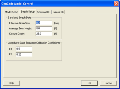
5. Click the tab for Beach Setup. For this example, the Effective Grain Size is 0.2 mm, the Average Berm Height is 8 feet, and the Closure Depth is 25 feet. K1 is 0.5, and K2 is 0.25.
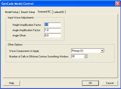
6. Go to the Seaward BC tab. Change the value of the Number of Cells in the Offshore Contour Smoothing Window under Other Options to 20. Keep all of the other defaults for this example.
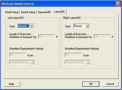
7. Click on the Lateral BC tab. Leave both the Left Lateral BC and Right Lateral BC as pinned.
Run GenCade
1. Save the project before running GenCade. Make sure the files are in the proper folder. After saving the project, the *.gen, *.shi, and *.wave files should appear.
2. Go to Edit->Preferences and click on File Locations in the SMS Preferences window. Scroll down to GenCade and make sure GenCade_v1_070 is the executable is listed (as of 24 November).
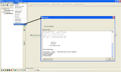
3. Go to GenCade->Run GenCade. This example should only take a few minutes to run. Click Exit to close the GenCade window.
View Results
1. Go to the folder that includes all of the saved input files. The output files (*.mql, *.mqr, *.mqn, *.off, *.slo, *.qtr, *.prt, and *.irv) should have been created during the simulation.
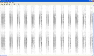
2. Open the *.slo file. Scroll down to the bottom of the file and ensure that the model ran for the entire simulation. If GenCade crashed during the simulation, "NaN" will replace the calculated shoreline output from the time of the crash until the end of the simulation. However, everything should be fine for this simple example.
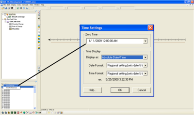
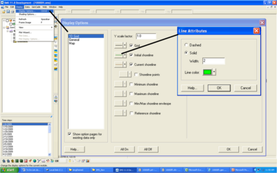
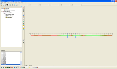
3. Drag the *.slo file into the SMS. Notice that a new window has opened on the screen which shows the time steps. Right click Time steps and select Time Settings. Change the Zero Time to 1/1/2009 12:00:00 AM. Also change the Display at: option under Time Display to Absolute Date/Time. Leave the Date Format and Time Format as the defaults. Click OK. Now the correct dates should be assigned to the time steps. Go to Display->Display Options. The Display Options window will open to the 1D Grid screen. Click on the button to the left of the words Initial Shoreline. This will open the Line Attributes window. The default line colors and widths are sometimes difficult to see. Change the line color and make the line thicker. Do the same with the Current Shoreline. Click OK. Make sure Shoreline is highlighted under GenCade Grid in the left panel. Click on 1/8/2009 under Time steps. Scroll through the dates to see the calculated shorelines.
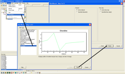
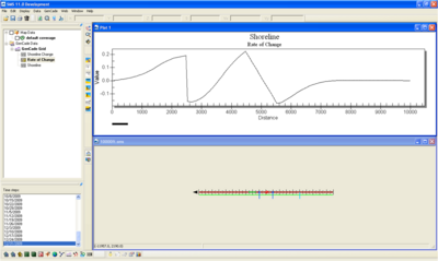
4. Go to Display->Plot Wizard. Click on Shoreline under Plot Type (Step 1 of 2). Click Next. Choose Active dataset under Dataset and Active time step under Time step. Select Finish. A new window should open which shows the shoreline at the final time step (12/31/2009). Please note the shoreline value is relative to the GenCade grid. This is the reason both the left most and right most cells have a value of 200. Also, the left side of the plot represents the left boundary condition. In this case, the left boundary condition is visually on the right side of the screen in the graphical window. Highlight the Rate of Change under GenCade Grid in the left panel. Notice the plot changes accordingly. Select Shoreline Change under GenCade Grid in the left panel. The plot will now show the amount of shoreline change between 1/1/2009 and 12/31/2009. Right click on the plot to change the axes titles, legend, and symbol size.
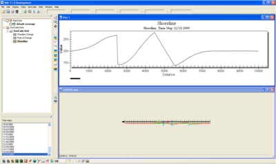
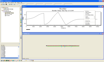
5. It may be necessary to make a plot with more detail using Microsoft Excel or similar tool. Open the *.prt file. Scroll down to SHORELINE CHANGE AFTER 1 YEARS. This section will list the shoreline position at each cell at the end of one year. Copy the values to Microsoft Excel. Please note that the values will need to be transposed before making the plot. In this case, the cell size is constant at 50 ft, so it is simple to determine the distance each cell is from the left boundary. The resulting plot should look similar to the plot developed in the Plot Wizard in the SMS. If this case had variable grid resolution, it would be necessary to open the *.shdx file and copy the values to the spreadsheet. Each of these values represent the size of an individual cell, so make sure to add the cell sizes together to get the distance from the left boundary.
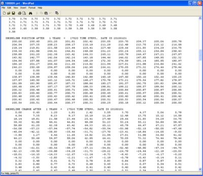
During calibration, the user will likely need to compare the final calculated shoreline to a measured shoreline. To do this, scroll down to the SHORELINE POSITION AFTER X YEARS (X is the final year in the simulation) in the *.prt file. Copy the values to the spreadsheet and transpose. These are the shoreline positions relative to the grid, so it is necessary to determine the measured shoreline positions relative to the grid. An easy way to do this is to return to the conceptual model. Make sure to save this as a new project before making any changes. Right click Map Data and select New Coverage. In the New Coverage window, scroll down and select GenCade. Drag the measured shoreline into the SMS as a *.cst file. Please see GenCade User's Guide for instructions. Click on the Select Feature Arc button and double-click on the arc. Make this arc the new initial shoreline. Right click on the New Coverage under Map Data and Convert to 1D Grid. The measured shoreline will become the initial shoreline. Save the project. Open the *.shi file. The measured shoreline is in the same format as the shoreline positions in the *.prt file. Copy these values to the spreadsheet. It is also necessary to copy the real initial shoreline positions to the spreadsheet. Subtract the initial shoreline positions from the final calculated shoreline positions and the measured shoreline positions. The plot will show the shoreline change for the calculated shoreline and the measured shoreline. The user will be able to see where the calculated shoreline is very different from the measured shoreline.
Zip File
The files for this example can be found here (File:GenCade example.zip).
The *.sms is also available in the zip file. To run the simulation, simply drag the *.sms project into the SMS. Save As a new project in a new location. Go to the new location and double-check that the locations for the *.shi and *.prt files are correct in the *.gen file. If these are correct, Run GenCade. The new results can be compared to the example results. This is a simple way to make sure GenCade is functioning correctly on a new machine.
A new project can also be started. After following each step in this section, the new results should be identical to the results in the zip file example.
Return to GenCade Main Page.