Model Coupling
Coupling Procedure

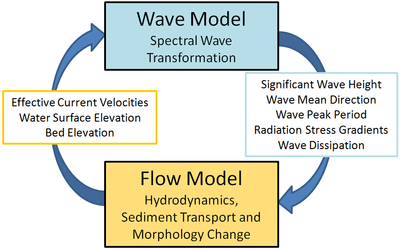
CMS-Flow and CMS-Wave can be run separately or coupled together using a process called steering (Figure 3.7). The variables passed from CMS-Wave to CMS-Flow are the significant wave height, peak wave period, wave direction, wave breaking dissipation, and radiation stress gradients. CMS-Wave uses the updated bathymetry (if sediment transport is turned on), water levels, and current velocities from CMS-Flow.

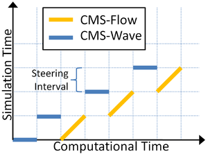
The time interval at which the CMS-Wave model is run is called the steering interval. Currently, the steering interval is constant and therefore the input spectra must be at constant intervals without any gaps. A schematic showing the steering process is shown in Figure 3.8 in which the simulations time is plotted as a function of the computational time.
In CMS versions less than 4.0, the steering process is controlled in the SMS interface using communication files because the CMS-Wave nd CMS-Flo models where separate executables. In CMS versions 4.0 and newer, both CMS-Flow and CMS-Wave are contained within a single executable (inline) and the steering process is controlled by an interval steering module. The advantages of the inline steering are that the model runs faster because there is no need to use communication files or reinitialize the models (memory allocation, variable initialization, etc.), makes the improvement and maintenance of the steering module easier for the developers, and also makes the code more portable to other operating systems. The inline steering process is as follows:
- CMS-Wave model is run the first two time steps and the wave information is passed to CMS-Flow. If specified, the surface roller model is run on the wave grid and the roller contributions to the radiation stresses are added to the wave radiation stresses.
- The wave height, period, wave dissipation, radiation stress gradients, and wave unit vectors are interpolated spatially from the wave grid to the flow grid.
- CMS-Flow is run until the next steering interval and interpolates the wave variables from during the simulation. At each flow time step, variables such as wave length and bottom orbital velocities are updated for wave-current interaction.
- Water levels, current velocities and bed elevations are estimated for the next wave time step and are interpolated from the flow grid to the wave grid.
- CMS-Wave is run again for the next time step.
- Step 2-7 are repeated until the end of the simulation.
Prediction of Water Levels and Currents
Because CMS-Wave requires the water surface elevation at times that are ahead of the hydrodynamics, the water surface elevation and currents. If the steering is relatively small (~<30 min), than the values from the previous time step may be used without significant error.
| (1) |
| (2) |
| (3) |
where n is the steering time step (CMS-Wave time step). However, in many coastal engineering projects it is desirable and common to use relatively large steering intervals of 2-3 hours and 3 hours is especially common since many wave buoy data products are at 3 hour intervals. Over large steering intervals, the change in water depth has the largest influence on the nearshore wave heights. Therefore, when using large steering intervals, it is desirable to make a better prediction of water levels than using the previous time step.
In cases where the relative surface gradients at any time are much smaller than the mean tidal elevation, a better approximation of water level may be obtained by decomposing the water level into
| (4) |
where is the mean water level, and is the component due to tidal, wave, and wind generated surface gradients. can be estimated from water level boundary conditions and is generally much larger, so may be neglected. For some cases in which the surface gradients do not vary significantly over time (open coast beach), the second term may be approximated as
| (5) |
Spatial Interpolation and Extrapolation
CMS allows the user to use the same or different grids for CMS-Flow and CMS-Wave. If the same grid is used, then no spatial interpolation is car-ried out. If different grids are used, then spatial interpolation is necessary in order to transfer information from one model grid to another model grid. The interpolation of wave variables from the CMS-Wave grid to the CMS-Flow grid is done using a combination of bilinear and linear triangular interpolation. Bilinear interpolation is applied at non-jointed cells (i.e. cells with 4 neighbors) and triangular interpolation at jointed cells (cells with more than 4 neighbors). If the extents of the CMS-Wave and CMS-Flow grids are different (e.g. if the CMS-Flow grid is smaller), then the extrapolation of variables is necessary in order to avoid boundary problems with the models. Different extrapolation methods are applied to different variables and are described below.
Water levels Water levels are extrapolated using a nearest neighbor interpolation over the entire domain, but not across land (dry) boundaries. This approach is more physically accurate than extrapolating only to a certain distance since water levels are controlled mainly by tides along the coast and the spatial variation is usually much smaller than the tidal range.
where is the water level at cell P, is the water level at the nearest neighbor, m is the CMS-Wave time step, and is the distance vector from cell P to N, and is an extrapolation distance. The subscripts flow and wave indicate the CMS-Flow and CMS-Wave grids, respectively.
Current Velocities Current velocities are extrapolated to a certain distance referred to as the extrapolation distance. A nearest neighbor extrapolation is applied to cells within that distance and multiplied by a cosine function to produce a smooth transition from the boundary to a value of zero:
where is the current velocity at the extrapolated cell, is the cur-rent velocity at the nearest neighbor, m is the CMS-Wave timestep, and is the distance vector from cell P to N, and is an extrapolation dis-tance.
Bed Elevations Extrapolating bed elevations from a boundary can lead to sharp changes in bathymetry in the wave model and instability problems in both the wave and flow models. Therefore, a plausible approach is to extrapolate the bed change
where is the bed elevation the extrapolated cell, is the bed elevation at the nearest neighbor, m is the CMS-Wave time step, and is the distance vector from cell P to N, and is in this case the flow grid extrapolation distance.
Significant Wave Height The significant wave height is extrapolated in the same way as the current velocities to a certain distance referred to as the extrapolation distance. A nearest neighbor extrapolation is applied to cells within that distance and multiplied by a cosine function to produce a smooth transition from the boundary to a value of zero:
where is the significant wave height velocity at the extrapolated cell, is the current velocity at the nearest neighbor, n is the CMS-Wave timestep, and is the distance vector from cell P to N, and is in this case the wave (right?) grid extrapolation distance.
Peak Wave Period The peak wave period is extrapolated in a similar way as the water levels using a nearest neighbor extrapolation over the entire domain, but not across land (dry) boundaries. This approach is more physically plausible than extrapolating to a finite distance and would produce zero wave pe-riods over the ocean domain (which is not physically meaningful).
Mean Wave Direction The mean wave direction is first converted to wave unit vectors and these unit vectors are extrapolated in space. Wave unit vectors are also extrapo-lated over the entire domain, except across land (dry) boundaries, without consideration of an extrapolation distance. This approach leads to more physically plausible results.
Temporal Interpolation and Prediction
Because CMS-Wave requires the water surface elevation at times that are ahead of the hydrodynamic model, the water surface elevation and cur-rents must be predicted for the CMS-Wave time step. If the steering is relatively small (<30 min), then the values from the last time step may be used without significant error.
where m is the CMS-Wave time step, n is the last CMS-Flow time step, and the subscript flow indicates the variables on the CMS-Flow grid. For many coastal engineering applications, it is desirable and common to use relatively large steering intervals of 2-3 hours. For large steering intervals, the change in water depth has the largest influence on the nearshore wave heights. Therefore, when using large steering intervals, it is desirable to make better predictions of water levels and not use the previous time step water levels. In cases where the relative surface gradients at any time are much smaller than the mean tidal elevation, a better approximation of water level may be obtained by decomposing the water level into
where is the mean water level and is a variation around the mean due to due to tidal, wave, and wind generated surface gradients. can be estimated from water level boundary conditions and is generally much larger, so may be neglected. The surface gradient term may be approx-imated as
For most coastal inlet applications, Equation 3-42 is a better representa-tion of the water surface elevation and is used as the default in CMS. After spatially interpolating the wave height, period, dissipation, and forcing onto the CMS-Flow grid, the variables are linearly interpolated in time. The wavelength, bottom orbital velocities, and mean wave-current bottom friction are then updated including current-wave interactions at each time step.
| Symbol | Description | Units |
|---|---|---|
| Water surface elevation | m |