Flow over a bump: Difference between revisions
m (→Setup) |
|||
| (6 intermediate revisions by one other user not shown) | |||
| Line 3: | Line 3: | ||
<font color=red>'''UNDER CONSTRUCTION'''</font> | <font color=red>'''UNDER CONSTRUCTION'''</font> | ||
== Setup == | == Setup == | ||
The spatial domain consists of a rectangular | The spatial domain consists of a rectangular domain with the bed elevation <math>z_b</math> given by | ||
\begin{equation} \tag{1} | |||
\begin{cases} | z_b = | ||
0, & \mbox{if } x<8 \\ | \begin{cases} | ||
0.2-0.05(x-10)^2, & \mbox{if } 8 \leq x \leq 12 \\ | 0, & \mbox{if } x<8 \\ | ||
0, & \mbox{if } x>8 \\ | 0.2-0.05(x-10)^2, & \mbox{if } 8 \leq x \leq 12 \\ | ||
\end{cases} | 0, & \mbox{if } x>8 \\ | ||
\end{cases} | |||
\end{equation} | |||
where | where <math>x</math> is the horizontal distance. | ||
Table 1. General Settings for Flow over a Bump | '''Table 1. General Settings for Flow over a Bump''' | ||
{|border="1" | {|border="1" | ||
|'''Parameter''' | |'''Parameter''' | ||
| Line 30: | Line 32: | ||
== Model Setup == | == Model Setup == | ||
[[Image:Bump_Grid.png|thumb|right|600px| Figure 1. Computational grid.]] | [[Image:Bump_Grid.png|thumb|right|600px| Figure 1. Computational grid.]] | ||
The computational domain is 25 m long and has a constant grid resolution of 0.1 m. A flux boundary condition is specified at the inflow boundary and a constant water level boundary condition is applied to the downstream boundary. An adaptive time between 0.1-1 s is applied. The computational time on a single processor is approximately | The computational domain is 25 m long and has a constant grid resolution of 0.1 m. A flux boundary condition is specified at the inflow boundary and a constant water level boundary condition is applied to the downstream boundary. An adaptive time between 0.1-1 s is applied. The computational time on a single processor is approximately 1 min. | ||
<br style="clear:both" /> | <br style="clear:both" /> | ||
| Line 41: | Line 43: | ||
Table 2. Goodness of fit statistics for the water elevation | Table 2. Goodness of fit statistics for the water elevation | ||
{|border="1" | {|border="1" | ||
|'''Statistic''' | |'''Statistic''' ||'''Value''' | ||
|'''Value''' | |||
|- | |- | ||
|RMSE | |RMSE || 0.0074 m | ||
| 0.0074 m | |||
|- | |- | ||
| | |NMAE || 0.0068 | ||
| 0.0068 | |||
|- | |- | ||
|R^2 | |R^2 || 0.991 | ||
| 0.991 | |||
|- | |- | ||
|Bias | |Bias || 0.0017 m | ||
| 0.0017 m | |||
|} | |} | ||
* For a definition of the goodness of fit statistics see [[Statistics | Goodness of fit statistics]]. | |||
<br style="clear:both" /> | <br style="clear:both" /> | ||
== References == | == References == | ||
*Caleffi, V., Valiani, A., and Zanni, A. (2003). "Finite volume method for simulating extreme flood events in | *Caleffi, V., Valiani, A., and Zanni, A. (2003). "Finite volume method for simulating extreme flood events in natural channels," Journal of Hydraulic Research, 41(2), 167-177. | ||
---- | ---- | ||
Latest revision as of 14:36, 16 July 2012
UNDER CONSTRUCTION
Setup
The spatial domain consists of a rectangular domain with the bed elevation given by \begin{equation} \tag{1}
 z_b =
 \begin{cases}
    0, & \mbox{if } x<8  \\
    0.2-0.05(x-10)^2, & \mbox{if } 8 \leq x \leq 12 \\
    0, & \mbox{if } x>8  \\
 \end{cases}
\end{equation}
where is the horizontal distance.
Table 1. General Settings for Flow over a Bump
| Parameter | Value |
| Discharge | 0.18 m^3/s |
| Downstream water level | 0.33 m |
| Bottom friction | None |
Model Setup
The computational domain is 25 m long and has a constant grid resolution of 0.1 m. A flux boundary condition is specified at the inflow boundary and a constant water level boundary condition is applied to the downstream boundary. An adaptive time between 0.1-1 s is applied. The computational time on a single processor is approximately 1 min.
Results
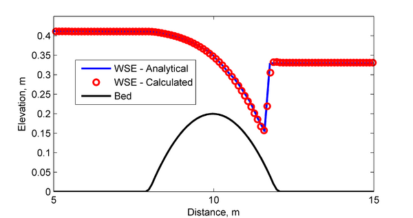
A comparison between the analytical solution for water levels is compared to the calculated water levels in Figure 2. As shown in the goodness of fit statistics, the model results agree well with the analytical solution. The minimum water level is captured well, however there is a small shift in the location of the water level drop over the bump toward the downstream direction.
Table 2. Goodness of fit statistics for the water elevation
| Statistic | Value |
| RMSE | 0.0074 m |
| NMAE | 0.0068 |
| R^2 | 0.991 |
| Bias | 0.0017 m |
- For a definition of the goodness of fit statistics see Goodness of fit statistics.
References
- Caleffi, V., Valiani, A., and Zanni, A. (2003). "Finite volume method for simulating extreme flood events in natural channels," Journal of Hydraulic Research, 41(2), 167-177.


