GenCade Output Files: Difference between revisions
mNo edit summary |
|||
| Line 1: | Line 1: | ||
{{TOC right}} | {{TOC right}} | ||
After running GenCade, several output files will be created in the designated folder. In GenCade Version 1.070, these files include *.prt, *.slo, *.qtr, *.off, *.mql, *.mqn, *.mqr, and *. | = Standard Output files = | ||
After running GenCade, several output files will be created in the designated folder. In GenCade Version 1.070, these files include *.prt, *.slo, *.qtr, *.off, *.mql, *.mqn, *.mqr, *.irv, *.vcc, and *.vcx. | |||
= Print file (*.prt) = | == Print file (*.prt) == | ||
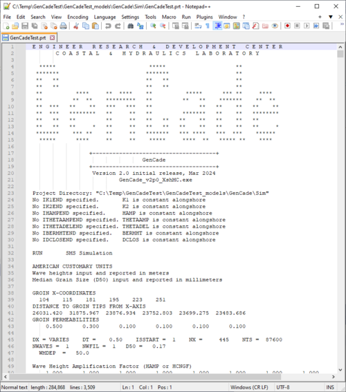
The *.prt is the print file, and it has a variety of information for the user. This file includes the initial shoreline position; the shoreline position, shoreline change, the breaking wave angle to the x-axis, the offshore wave angle to the x-axis, the breaking wave height, the offshore wave height, the gross transport volume, the net transport volume, the transport volume to the left, and the transport volume to the right after each year in the simulation; the mean net annual transport, mean annual transport to the left, mean annual transport to the right, the calculated seawardmost shoreline position, the calculated landwardmost shoreline position, the calculated representative offshore contour position, the average undiffracted breaking wave heights, the average undiffracted breaking wave angle to the shoreline, and the average longshore transport rate based on undiffracted waves. | The *.prt is the print file, and it has a variety of information for the user. This file includes the initial shoreline position; the shoreline position, shoreline change, the breaking wave angle to the x-axis, the offshore wave angle to the x-axis, the breaking wave height, the offshore wave height, the gross transport volume, the net transport volume, the transport volume to the left, and the transport volume to the right after each year in the simulation; the mean net annual transport, mean annual transport to the left, mean annual transport to the right, the calculated seawardmost shoreline position, the calculated landwardmost shoreline position, the calculated representative offshore contour position, the average undiffracted breaking wave heights, the average undiffracted breaking wave angle to the shoreline, and the average longshore transport rate based on undiffracted waves. | ||
[[Image:prt.png| | [[Image:prt.png|500px|thumb|left|Figure 1. Example *.prt]] | ||
<br style="clear:both" /> | <br style="clear:both" /> | ||
= Shoreline position output file (*.slo) = | == Shoreline position output file (*.slo) == | ||
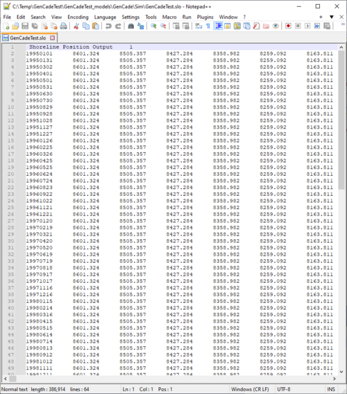
The *.slo is the shoreline position output. Each row in the document represents one time step in the simulation. The shoreline position at each cell is listed in the columns for each time step. This shoreline position is relative to the grid (not the initial shoreline). This file can be read into the SMS to see the shoreline for each time step. | The *.slo is the shoreline position output. Each row in the document represents one time step in the simulation. The shoreline position at each cell is listed in the columns for each time step. This shoreline position is relative to the grid (not the initial shoreline). This file can be read into the SMS to see the shoreline for each time step. | ||
[[Image:slo.png| | [[Image:slo.png|500px|thumb|left|Figure 2. Example *.slo]] | ||
<br style="clear:both" /> | <br style="clear:both" /> | ||
= Net annual transport rate file (*. | == Net annual transport rate file (*.qtr) == | ||
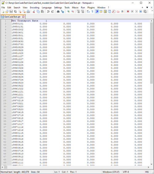
The net annual transport rate for each cell at each time step is included in the file. | The net annual transport rate for each cell at each time step is included in the file. | ||
[[Image:qtr.png| | [[Image:qtr.png|500px|thumb|left|Figure 3. Example *.qtr]] | ||
<br style="clear:both" /> | <br style="clear:both" /> | ||
= Offshore contour file (*.off) = | == Offshore contour file (*.off) == | ||
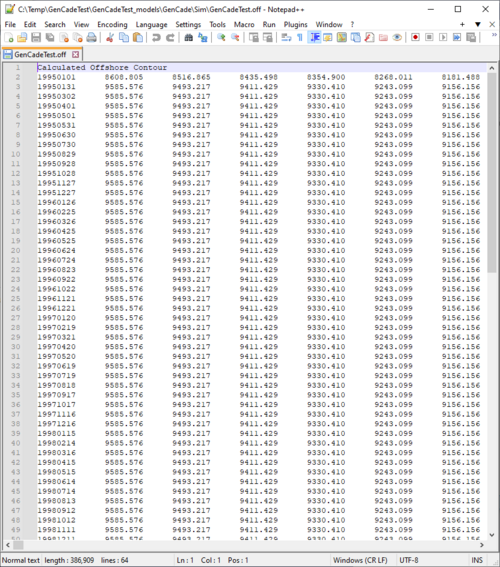
The *.off file is the offshore contour. This file is the output of the calculated offshore contour (not regional contour) at every output time step. | The *.off file is the offshore contour. This file is the output of the calculated offshore contour (not regional contour) at every output time step. | ||
[[Image:off.png| | [[Image:off.png|500px|thumb|left|Figure 4. Example *.off]] | ||
<br style="clear:both" /> | <br style="clear:both" /> | ||
= Mean annual transport files (*.mqn, *.mqr, *.mql) = | == Mean annual transport files (*.mqn, *.mqr, *.mql) == | ||
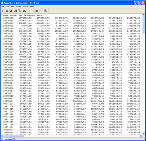
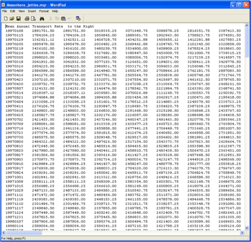
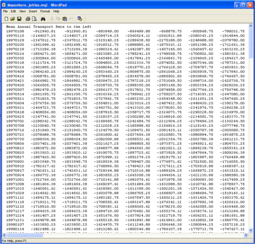
The mean annual transports are included in the *.mqn, *.mqr, and *.mql. Mean annual net transport is *.mqn, *.mqr is mean annual transport to the right, and *.mql is mean annual transport to the left. | The mean annual transports are included in the *.mqn, *.mqr, and *.mql. Mean annual net transport is *.mqn, *.mqr is mean annual transport to the right, and *.mql is mean annual transport to the left. | ||
[[Image:mqn.png| | [[Image:mqn.png|500px|thumb|left|Figure 5. Example *.mqn for net total]] | ||
<br style="clear:both" /> | <br style="clear:both" /> | ||
[[Image:mqr.png| | [[Image:mqr.png|500px|thumb|left|Figure 6. Example *.mqr for transport to right]] | ||
<br style="clear:both" /> | <br style="clear:both" /> | ||
[[Image:mql.png| | [[Image:mql.png|500px|thumb|left|Figure 7. Example *.mql for transport to left]] | ||
<br style="clear:both" /> | <br style="clear:both" /> | ||
= Inlet shoal volume file (*.irv) = | == Inlet shoal volume file (*.irv) == | ||
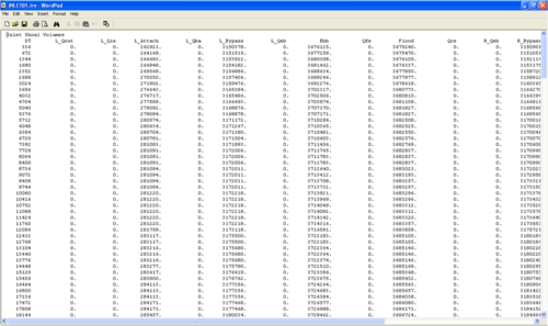
The inlet shoal volumes for each time step in the simulation are included in the *.irv files. There is one *.irv file for each inlet in the grid. In older files, the files are named INLET01.irv, INLET02.irv. More recently, the *.irv file name includes the user specified inlet name. | The inlet shoal volumes for each time step in the simulation are included in the *.irv files. There is one *.irv file for each inlet in the grid. In older files, the files are named INLET01.irv, INLET02.irv. More recently, the *.irv file name includes the user specified inlet name. | ||
[[Image:irv.png| | [[Image:irv.png|500px|thumb|left|Figure 8. Example *.irv]] | ||
<br style="clear:both" /> | <br style="clear:both" /> | ||
== Volume change per cell file (*.vcc) == | |||
[[Image:vcc.png|500px|thumb|left|Figure 8. Example *.vcc]] | |||
<br style="clear:both" /> | |||
== Volume change per linear distance (*.vcx) == | |||
[[Image:vcx.png|500px|thumb|left|Figure 8. Example *.vcx]] | |||
<br style="clear:both" /> | |||
= Cross-Shore Output files = | |||
After running GenCade with Cross-shore enabled, several output files will be created in the designated folder. These are available in GenCade Version 2.0 and the files include *.hso, *.ktv, *.xsh, *.wvo, *.xshqw, *.xshqc, *.xshqd, and *.BFslp. | |||
* .hso - Breaking Wave Height | |||
* .ktv - Transmission coefficient Kt | |||
* .xsh - Cross-shore Transport Rate | |||
* .wvo - Wave Output at the middle of the shoreline | |||
* .xshqw - Cross-shore Transport Rate due to waves | |||
* .xshqc - Cross-shore Transport Rate due to currents | |||
* .xshqd - Cross-shore Transport Rate due to gravity | |||
* .BFslp - Estimated Beachface slope by Cross-shore Transport model | |||
Return to [[GenCade|GenCade Main Page.]] | Return to [[GenCade|GenCade Main Page.]] | ||
Revision as of 19:05, 10 January 2024
Standard Output files
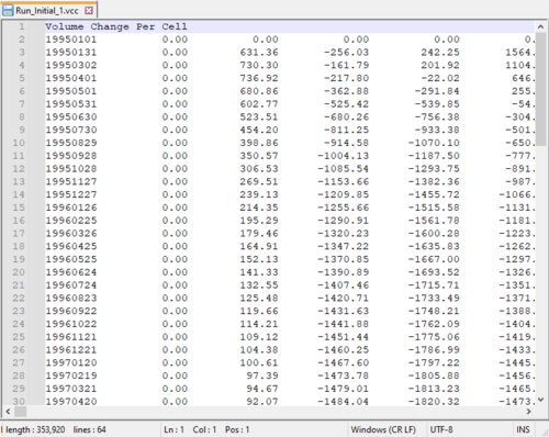
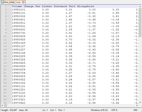
After running GenCade, several output files will be created in the designated folder. In GenCade Version 1.070, these files include *.prt, *.slo, *.qtr, *.off, *.mql, *.mqn, *.mqr, *.irv, *.vcc, and *.vcx.
Print file (*.prt)
The *.prt is the print file, and it has a variety of information for the user. This file includes the initial shoreline position; the shoreline position, shoreline change, the breaking wave angle to the x-axis, the offshore wave angle to the x-axis, the breaking wave height, the offshore wave height, the gross transport volume, the net transport volume, the transport volume to the left, and the transport volume to the right after each year in the simulation; the mean net annual transport, mean annual transport to the left, mean annual transport to the right, the calculated seawardmost shoreline position, the calculated landwardmost shoreline position, the calculated representative offshore contour position, the average undiffracted breaking wave heights, the average undiffracted breaking wave angle to the shoreline, and the average longshore transport rate based on undiffracted waves.
Shoreline position output file (*.slo)
The *.slo is the shoreline position output. Each row in the document represents one time step in the simulation. The shoreline position at each cell is listed in the columns for each time step. This shoreline position is relative to the grid (not the initial shoreline). This file can be read into the SMS to see the shoreline for each time step.
Net annual transport rate file (*.qtr)
The net annual transport rate for each cell at each time step is included in the file.
Offshore contour file (*.off)
The *.off file is the offshore contour. This file is the output of the calculated offshore contour (not regional contour) at every output time step.
Mean annual transport files (*.mqn, *.mqr, *.mql)
The mean annual transports are included in the *.mqn, *.mqr, and *.mql. Mean annual net transport is *.mqn, *.mqr is mean annual transport to the right, and *.mql is mean annual transport to the left.
Inlet shoal volume file (*.irv)
The inlet shoal volumes for each time step in the simulation are included in the *.irv files. There is one *.irv file for each inlet in the grid. In older files, the files are named INLET01.irv, INLET02.irv. More recently, the *.irv file name includes the user specified inlet name.
Volume change per cell file (*.vcc)
Volume change per linear distance (*.vcx)
Cross-Shore Output files
After running GenCade with Cross-shore enabled, several output files will be created in the designated folder. These are available in GenCade Version 2.0 and the files include *.hso, *.ktv, *.xsh, *.wvo, *.xshqw, *.xshqc, *.xshqd, and *.BFslp.
- .hso - Breaking Wave Height
- .ktv - Transmission coefficient Kt
- .xsh - Cross-shore Transport Rate
- .wvo - Wave Output at the middle of the shoreline
- .xshqw - Cross-shore Transport Rate due to waves
- .xshqc - Cross-shore Transport Rate due to currents
- .xshqd - Cross-shore Transport Rate due to gravity
- .BFslp - Estimated Beachface slope by Cross-shore Transport model
Return to GenCade Main Page.
