Long wave propagation: Difference between revisions
No edit summary |
|||
| Line 16: | Line 16: | ||
= Model Setup = | = Model Setup = | ||
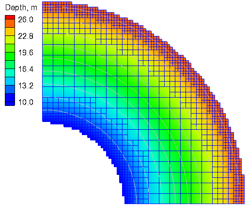
[[Image:QA_Depth_8km.png|thumb|right|600px| Figure 1. Quarter Annulus]] | |||
A Cartesian grid is used with two levels of refinement. The computational grid is shown in Figure 1. The general model settings are shown in Table 2. | A Cartesian grid is used with two levels of refinement. The computational grid is shown in Figure 1. The general model settings are shown in Table 2. | ||
| Line 35: | Line 36: | ||
|} | |} | ||
<br style="clear:both" /> | |||
= Results = | = Results = | ||
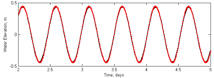
The figure below shows a time series of water levels at the inner edge of the model domain. The goodness of fit statistics are listed in the below. The model accurately predicts the wave phase but slightly overestimates the amplitude by approximately 0.01 m. | The figure below shows a time series of water levels at the inner edge of the model domain. The goodness of fit statistics are listed in the below. The model accurately predicts the wave phase but slightly overestimates the amplitude by approximately 0.01 m. | ||
Revision as of 23:28, 3 March 2011
Analytical Solution
The purpose of this verification test is to assess the model performance in simulating long wave propagation. The case is also useful for testing the model performance and symmetry for a non-rectangular domain. The test case consists of a quarter annulus with a linear bed elevation in the radial direction. The inner radius is 60.96 km (200,000 ft), and the outer radius is 152.4 km (500,000 ft). The analytical is given by Lynch and Gray (1978).
Table 1. General Settings for Flow over a Bump
| Parameter | Value |
| Deepwater Tidal Amplitude | 0.3048 m |
| Tidal Period | 12.42 hrs (M2) |
| Bottom friction | None |
| Horizontal eddy viscosity | None |
Model Setup
A Cartesian grid is used with two levels of refinement. The computational grid is shown in Figure 1. The general model settings are shown in Table 2.
Table 2. General Settings for Flow over a Bump
| Parameter | Value |
| Time step | 600 sec (10 min) |
| Ramp period | 24 hrs |
| Simulation time | 120 hrs |
| Grid resolution | 2-8 km |
| Number of active ocean cells | 1160 |
| Wall friction | Off |
Results
The figure below shows a time series of water levels at the inner edge of the model domain. The goodness of fit statistics are listed in the below. The model accurately predicts the wave phase but slightly overestimates the amplitude by approximately 0.01 m.
Table 3. Goodness of fit statistics for the water elevation
| Statistic | Value |
| RMSE | 0.014 m |
| RMAE | 0.028 |
| R^2 | 0.999 |
| Bias | 0.003 m |
References
- Lynch, D.R., and Gray, W.G. (1978). "Analytical solutions for computer flow model testing," J. Hydraulics Division, 104, 1409-28.

