User Guide 003: Difference between revisions
No edit summary |
No edit summary |
||
| Line 120: | Line 120: | ||
Figure 2 27. Bottom Friction Dataset specification via the Input tab of the CMS-Flow Model Control window in SMS 11.0 | Figure 2 27. Bottom Friction Dataset specification via the Input tab of the CMS-Flow Model Control window in SMS 11.0 | ||
[[File:fig_2- | [[File:fig_2-28a.png]] | ||
Figure 2-28. Bottom friction specification via the ''Flow'' tab of the ''CMS-Flow Model Control'' window in SMS 11.1 | Figure 2-28. Bottom friction specification via the ''Flow'' tab of the ''CMS-Flow Model Control'' window in SMS 11.1 | ||
| Line 131: | Line 131: | ||
[[File:fig_2-29.png]] | [[File:fig_2-29.png]] | ||
Figure 2 29. Three SMS Project Explorer showing the Manning's ''n'', Bottom Friction Coefficient and Roughness Height datasets. | Figure 2-29. Three SMS Project Explorer showing the Manning's ''n'', Bottom Friction Coefficient and Roughness Height datasets. | ||
=Bottom Friction Value= | =Bottom Friction Value= | ||
| Line 144: | Line 144: | ||
In the presence of waves, the mean (short-wave averaged) bottom shear stress which is used in the momentum equations is enhanced: | In the presence of waves, the mean (short-wave averaged) bottom shear stress which is used in the momentum equations is enhanced: | ||
{{Equation|<math> \tau_{bi} = \lambda_{wc}\ | {{Equation|<math> \tau_{bi} = \lambda_{wc}\tau_{ci}</math>|2-4}} | ||
where | where | ||
<math>\tau_{bi}</math> = combined wave and current mean bed shear stress [Pa] | <math>\tau_{bi}</math> = combined wave and current mean bed shear stress [Pa] | ||
<math> \lambda_{wc}</math> = nonlinear bottom friction enhancement factor (<math>\lambda_{wc} \geq 1 ) [-] | |||
<math> \lambda_{wc}</math> = nonlinear bottom friction enhancement factor (<math>\lambda_{wc} \geq 1 </math> ) [-] | |||
<math> \tau{ci}</math>= current-related bed shear stress [Pa]. | |||
The nonlinear bottom friction enhancement factor (<math>\lambda_{wc}</math> ) is calculated us-ing one of the following formulations (name abbreviations are given in parenthesis): | The nonlinear bottom friction enhancement factor (<math>\lambda_{wc}</math> ) is calculated us-ing one of the following formulations (name abbreviations are given in parenthesis): | ||
Revision as of 18:58, 1 May 2015
Hydrodynamics
The hydrodynamic parameters are divided into different groups: Water Properties, Bottom Friction, Wall Friction, Eddy Viscosity, Wave Mass Flux, and Wind and Atmospheric Pressure. Each group is discussed in detail in the following sections. A brief over is provided on what the options and parameters are, where to change them and other pertinent information.
Figure 2-23. Flow tab of th CMS-Flow Model Control window in SMS 11.1
Water Properties
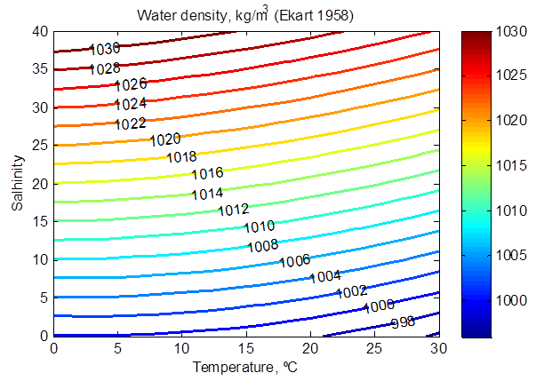
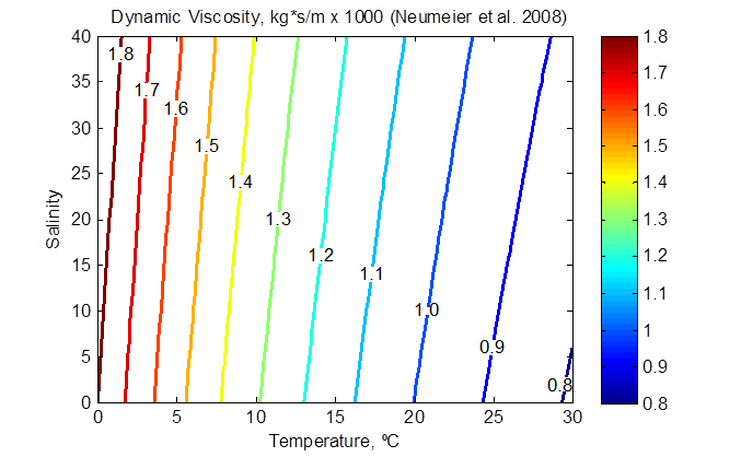
The properties of sea water are a function of temperature, salinity (i.e. dissolved minerals) and pressure. The water density and dynamic viscosity (kinematic viscosity times the water density) are shown in the following two figures as a function of water temperature and salinity.
Figure 2 24. Water density as a function of temperature and salinity (at atmospheric pressure).
Figure 2 25. Water dynamic viscosity as a function of temperature and salinity (at atmospheric pressure).
CMS uses the water density and viscosity in various hydrodynamic and sediment transport calculations. The water density and viscosity are as-sumed to be constant and can be either user-specified or calculated inter-nally based on the water temperature and salinity. The water temperature must always be specified, while either the water density or salinity need to be specified. If the salinity is not specified, then it is calculated from the water density. The salinity value used to calculate the water density and viscosity are independent of the salinity transport (initial condition and time-varying solution). Below is a table describing the CMS cards related to the specification of the water properties.
table 2-23
In SMS 11.1 and earlier versions, only the option to specify the water density and temperature were available (see Figure 2 23). Below is an example of the CMS cards used to specify the water density and temperature are specified as when using the SMS interface. The default salinity value of 35 ppt is used to estimate the water viscosity. Therefore, if the user wishes to simulate a fresh water location, the salinity should also be modified.
Example 2-8
If the user wants the model to calculate the water density based on the water temperature and salinity, or to change the default salinity value used in the water density and viscosity calculations, then the user must manually edit the CMS-Flow Control File. Below is an example where the Card file is manually modified (advanced) and the water temperature and salinity specified.
example 2-9
Notes
- 1. CMS uses a constant density, and kinematic viscosity. The water density and kinematic viscosity can be either specified are calculated based on the water temperature and salinity. The salinity value used in the water properties section is independent of the salinity transport initial condition and solution.
- 2. The kinematic viscosity and water density y are used in the many of the sediment transport calculations.
- 3. The water properties are NOT calibration parameters and should be estimated as best as possible.
- 4. All water properties are written in the CMS_Diag.txt file for the user’s reference.
Coriolis
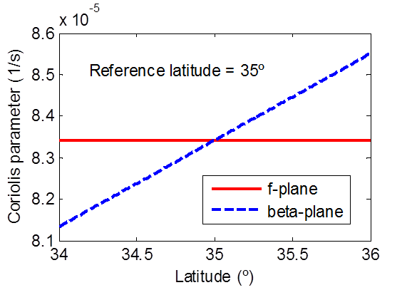
The Coriolis force is a fictitious force which arises from the earth’s rotation (Coriolis 1832). The Coriolis parameter is given by . Here = 7.29 x 10⁻⁵ rad/s is the earth’s angular velocity of rotation and is the latitude in degrees. Since the CMS uses a Cartesian coordinate system, the Coriolis parameter is approximated using either a constant (f-plane) or linearly varying (beta-plane). In the case of the f-plane approximation the constant value is based on the average-latitude of the domain as . In the case of the beta-plane approximation a linearly varying Coriolis parameter is used where the subscript a indicates the average-latitude of the active computational cells, y is the linear northward distance, and is a linear coefficient given by , in which RE is the earth radius. The average latitude can either be automatically computed when a non-local horizontal projection has been set or it may also be specified in the interface. Below is an example of the Coriolis parameter variation (reference latitude is 35º).
Figure 2-26. Example of the Coriolis parameter as a function of latitude using the f-plane and beta-plane approximations.
The table below describes the card used to specify the Coriolis approximation.
table 2-24
Below are two examples of how to specify the Coriolis parameter options:
example 2-10
example 2-11
Notes
- 1. Independently of whether the f-plane or beta-plane approximation is used to calculate the Coriolis parameter, the average latitude is needed. The average latitude can be either estimated based on the grid projection or specified by the user.
- 2. The Coriolis parameter can be turned off (set to zero) by setting the “Average latitude for Coriolis” to “User specified” and entering 0.0 (see Figure 2-23).
- 3. The Coriolis parameter is NOT a calibration parameter. It is recommended to use the Coriolis parameter for all regional scale applications. For small project scale applications, the effects of the Coriolis parameter are less important.
Bottom Friction
The bed roughness may be may specified using one of the following pa-rameters:
- 1. Manning’s n coefficient (n) [s/m1/3]
- 2. Bottom friction coefficient (cb) [-]
- 3. Roughness height (Nikuradse roughness) (ks) [m]
The Manning’s n coefficient (also referred to as Gauckler-Manning coefficient) was originally first developed for open channel flow (Gauckler 1867). If the Manning’s coefficient is specified, the bed friction coefficient is calculated internally at each time step from (Soulsby 1997)
| (2-2) |
If the input roughness is specified as a roughness height, the bed friction coefficient is calculated at each time step as (Graf and Altinakar 1998)
| (2-3) |
(2 3) where = 0.4 is Von Karman constant, and z0 is the bed roughness length which is related to the Nikuradse roughness () by ) (hydraulically rough flow).
Table 2-25 shows mean roughness heights from a large number of field measurements over natural sea beds.
table 2-25
table 2-26
Notes
- 1. The input roughness parameter is held constant throughout the simulation and not updated at each time step as a function of the hydrodynamics, bed composition, and bedforms. This is a common engineering approach which can be justified by the lack of data to initialize the bed composition and the large error in estimating the bed composition evolution and bedforms. In addition using a constant bottom roughness simplifies the model calibration. In future versions of CMS, the option to automatically estimate the bed roughness from the bed composition and bedforms will be added.
- 2. The bed roughness used for hydrodynamics may not be the same as that which is used for the sediment transport calculations because each sediment transport formula was developed and calibrated using specific methods for estimating bed shear stresses or velocities, and these cannot be easily changed. In the case of the Lund-CIRP transport formula the bed roughness is calculated as the sum of grain, transport, and bedform roughness’s.
- 3. The Manning’s coefficient should not be confused with the Manning’s number used by other models. The two are related by n = M-1 .
Bottom Friction Dataset
The bottom roughness may be specified using a grid dataset referred to as the Bottom Friction Dataset. The dataset contain spatially variable or constant values and is the most general way of specifying the bed roughness. A description of the CMS-Flow cards related to the Bottom Friction Dataset are shown in the table below.
table 2-27
example 2-12
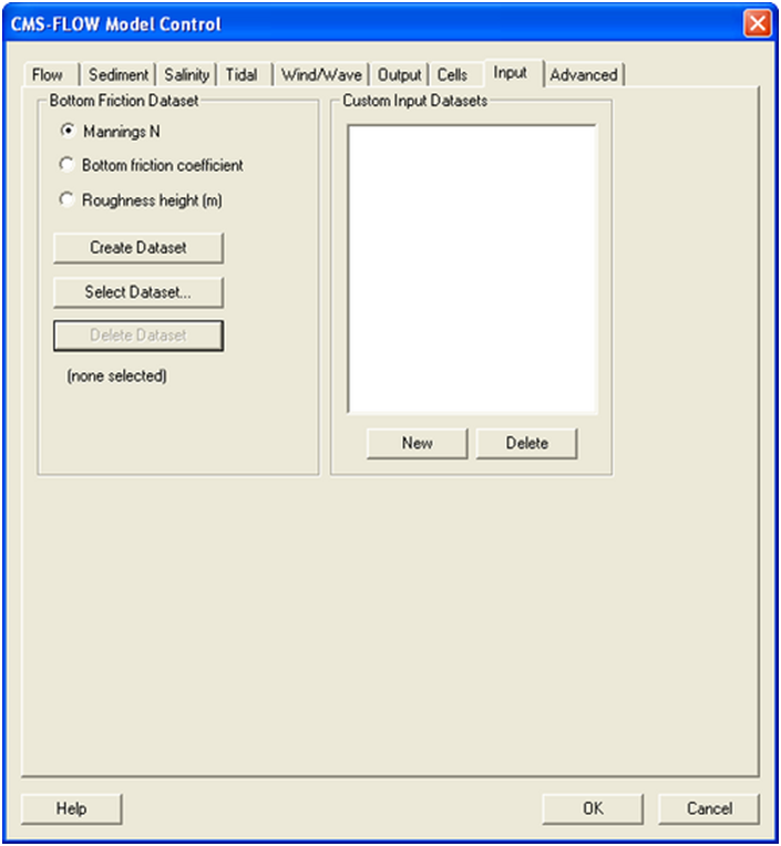
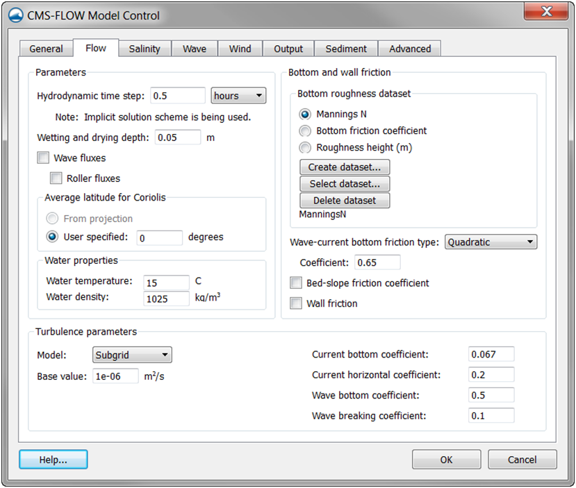
In SMS versions 10.1 and earlier, the bottom roughness was specified us-ing the Manning's n coefficient in the Cells tab of the CMS-Flow Model Control window. In SMS 11.0 the bottom roughness is specified in the Bottom Friction Dataset section of within the Input tab of the CMS-Flow Model Control window (see Figure 2-27). The Bottom Friction Dataset is specified at every computational (ocean) cell and is required for each model simulation. In SMS 11.1, the bottom friction dataset is specified in the Flow tab of the CMS-Flow Model Control window (see Figure 2 23). As in SMS 11.0, the bottom roughness can be specified as a roughness height, bottom friction coefficient, or in Manning's n coefficient.
Figure 2 27. Bottom Friction Dataset specification via the Input tab of the CMS-Flow Model Control window in SMS 11.0
Figure 2-28. Bottom friction specification via the Flow tab of the CMS-Flow Model Control window in SMS 11.1
Creating a Bottom Friction Dataset
Each time a new CMS-Flow simulation is created a bottom friction (roughness) dataset needs to be created using the Create Dataset button. The bottom friction parameter (related to Manning n) is spatially varying (cell-specific) over the grid domain. The default value upon grid creation is 0.025. At times a user may desire to represent locations where added friction is needed due to structures, vegetation, or increased turbulence due to rapid changes in current speed. Once the Bottom Friction Dataset is created and the CMS-Flow Model Control window closed, a new auxiliary dataset will appear in the SMS Project Explorer (see Figure 2-29).
Figure 2-29. Three SMS Project Explorer showing the Manning's n, Bottom Friction Coefficient and Roughness Height datasets.
Bottom Friction Value
Additional advanced cards (in Table 2-28) are available for setting the bottom friction to a constant for the whole grid. These cards are useful for running sensitivity analysis for a wide range of values in cases which can be approximated with a single constant bottom friction value.
table 2-28
example 2-13
Wave-enhanced Bottom Friction In the presence of waves, the mean (short-wave averaged) bottom shear stress which is used in the momentum equations is enhanced:
| (2-4) |
where
= combined wave and current mean bed shear stress [Pa]
= nonlinear bottom friction enhancement factor ( ) [-] = current-related bed shear stress [Pa].
The nonlinear bottom friction enhancement factor ( ) is calculated us-ing one of the following formulations (name abbreviations are given in parenthesis):
- 1. Wu et al. (2010)quadratic formula (QUAD )
- 2. Soulsby (1995) empirical two-coefficient data fit (DATA2)
- 3. Soulsby (1995) empirical thirteen-coefficient data fit (DATA13)
- 4. Fredsoe (1984) analytical wave-current boundary layer model (F84)
- 5. Huynh-Thanh and Temperville (1991) numerical wave-current boundary layer model (HT91)
- 6. Davies et al. (1988) numerical wave-current boundary layer model (DSK88)
- 7. Grant and Madsen (1979) analytical wave-current boundary layer model ( GM79)
For further details on the above methods, the reader is referred to the above references. The default is a simple quadratic formula but can be changes using the Advanced Card described in Table 2-29.
table 2-29
example 2-14
Bed-slope Friction Factor
The bed slope friction factor accounts for the increased surface area over sloping beds as compared to the horizontal area. This feature may be turned ON or OFF through the Advanced Card described in
table 2-30
example 2-15




![{\displaystyle c_{b}={\big [}{\frac {\kappa }{ln(z_{0}/h)+1}}]^{2}}](https://en.wikipedia.org/api/rest_v1/media/math/render/svg/2cd5e0366e116a23154d34322c3b7797cb20d288)


