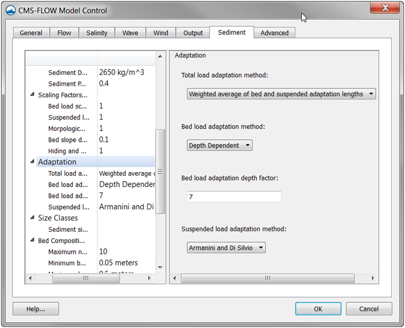
Figure 2-87. Example of the total load adaptation length specification within the Adaptation section within the Sediment tab of the CMS-Flow Model Control window in SMS 11.1.

Example 2-80. Total load adaptation length as the weighted averaged of the bed and suspended load lengths

ADAPTATION_METHOD_TOTAL WGHT_AVG_BED_SUSP_LENGTH ADAPTATION_METHOD_BED DEPTH_DEPENDENT ADAPTATION_DEPTH_FACTOR_BED 7.0 !dimensionless ADAPTATION_METHOD_SUSPENDED ARMANINI_DISILVIO

Hard Bottom Specification

Although the hard bottom dataset can be edited (when it’s the active da-taset) by selecting a cell (or group of cells) and changing the scalar (S) value in the Edit Window, an user-friendly window exists which provides specification options. With the Select Grid Cell tool active, make a selection, right click to bring up the tool menu and choose the Specify Hard Bottom... option. This will open the CMS-Flow Hard Bottom Specification window.

The following options are provided in the Hard Bottom Specification window:

• Use bathymetric cell depth - Sets the cell hard bottom depth to be the cell geometry value thereby creating an exposed non-erodible condition. If multiple cells were selected, then each cell will use its respective bathymetric depth.

• Specified distance below bathymetric cell depth - Sets the cell hard bottom depth to be the cell geometry value plus the specified distance thereby creating a sediment-covered non-erodible condition. The distance is limited to positive values to ensure the hard bottom depth is greater than the geometry value. The cell can provide sediment for transportation, however, the amount of erosion is limited. If multiple cells were selected, then each cell will use its respective bathymetric depth.

• Specified depth - Sets the cell hard bottom depth to the specified depth thereby creating a sediment-covered non-erodible condition similar to specified distance. The depth is limited to greater than the geometry value. If multiple cells were selected, then the depth is limited to greater than the largest geometry value and all cells will have the same value.

• Unspecified - Resets to an inactive hard bottom condition. The cell hard bottom depth is set to the CMS-Flow null value. If multiple cells were selected, then all cells will be reset.

If no cells are selected when opening the Hard Bottom Specification win-dow, then all computational (ocean) cells will be used. If a selection of only non-computational cells, then specification cannot occur. If a selection contains computational and non-computational cells, then the specification will only apply to the computational cells.

If multiple computational cells with differing specifications are selected, the window will not display a selected specification type and the OK button will be disabled. This is to protect the previous specifications from being overwritten by mistake. The OK button will be enabled when an option is selected. The minimum hard bottom depth of the multiple computational cells selected will be displayed in the Depth edit field and the minimum hard bottom depth minus the maximum geometry depth of the multiple computational cells selected will be displayed in the Distance edit field.

Display Options

The hard bottom dataset (when it’s the active dataset) will only display the cells with hard bottom specified if the Ocean cell display option is turned on. Inactive hard bottom cells are not displayed.

CMS-Flow includes hard bottom symbols to differentiate specifications. On the Cartesian Grid page of the Display Options window (when CMS-Flow is the active model), the Hard bottom symbols check box controls the display of symbols that will appear in hard bottom cells (even if the hard bottom dataset is not active). If this is turned on, then the user must be aware of the individual symbol settings accessed by clicking on the Options... button. The Options... button displays the CMS-Flow Hard Bottom Symbols window.

Hard bottom symbols can be selected for three hard bottom specification types:

• Non-erodible - Displayed in exposed hard bottom cells (cell hard bottom depth is equal to cell bathymetric depth).

• Erodible to specified depth - Displayed in sediment-covered hard bottom cells (cell hard bottom depth is greater than cell bath-ymetric depth).

• Invalid specification - Displayed in hard bottom cells where the hard bottom depth is less than cell bathymetric depth (the geometry is below the erosion limit).

If the Hard bottom symbols check box is turned off, no symbols will be displayed and the individual settings cannot be accessed, however, the individual settings will not be changed.

Bed Slope Term

The bed slope term accounts for the effect of gravity on sloped beds. The larger the bed slope coefficient, the more sediment tends to move downslope, thus smoothing the solution. The CMS-Flow used to specify the slope coefficient is described in the table below. The bed slope coeffi-cient is set in the Sediment tab of the CMS-Flow Model Control window in SMS 11.0.

Table 2-84. CMS card used to specify the sediment bed slope diffusion coefficient

Input	Format	Notes
Sediment Bed Slope Diffusion Coefficient	[card=SLOPE_COEFFICIENT] [name=SedBedSlopeCoeff, type=float, default=0.1, range=(0.0>=SedBedSlopeCoeff<5.0), typical=(0.1>SedBedSlopeCoeff<1.0)]	Sets the bed slope coefficient which controls enters a diffusion term which moves sediment down slope

Example 2 81. Specifying the sediment bed slope coefficient.

SLOPE_COEFFICIENT 0.1 !Dimensionless

=Note=:

• A constant bed slope coefficient is used spatially, temporally and for all sediment size classes.

• Increasing the bed slope coefficient will increase the smoothing of the bed.

• The measured morphology change can be used to calibrate this pa-rameter. However, its effect is less significant than the capacity transport formula and scaling factors.

Total-Load Correction Factor

The total-load correction factor accounts for the nonuniform vertical pro-file of sediment concentration and current velocity and produces temporal lag between the flow and sediment transport. The factor is used in the nonequilibrium total load sediment transport formula.

Table 2-85. CMS-Flow cards related to the total load correction factor.

Input	Format	Notes
Total load Correction Factor	[card=TOTAL_LOAD_CORR_FACTOR_CONSTANT, SMS_ver=none, CMS_ver=(>4.00.00)] [name=SedTotalCorrFac, type=float, default=none, optional=true, typical=(0.3>SedTotalCorrFac<1.0)]	Sets the total load correction factor to a constant.
Concentration Profile [cards=CONCENTRATION_PROFILE] [name=ConcPro, type=char, options=(LUND-CIRP,VAN_RIJN, EXPONENTIAL,ROUSE), default=EXPONENTIAL, exlusion=SedTotalCorrFac] Selects the concentration profile to be used either in the equilibrium A-D or NET models. In the A-D model, it is used to estimate the near bed concentration, whereas in the NET, it is used in the total-load correction factor.

Example 2-82. Specifying a constant total-load correction factor.

TOTAL_LOAD_CORR_FACTOR_CONSTANT 0.7 !Dimensionless

=Note=:

• The total load correction factor is only used for the total-load non-equilibrium transport model (NET).

• Computing the total-load correction factor based on the sediment concentration and current velocity profiles increases slightly the computational time but is almost negligible.

=Recommendations=:

• It is NOT recommended to use the total-load correction factor as a calibration factor.

Bed Composition

Single-sized Sediment Transport

In the case of single-sized sediment transport the bed is usually assumed to be uniform and variations in the bed composition are ignored. In CMS, the option is provided to use a unique approach which the bed composi-tion is allowed to be different from the single transported grain size and the bed composition is considered in hiding and exposure corrections to the sediment transport. The approach works well for cases where the bed is uniform and well sorted with local patches of coarse material such as shell hash. In this approach the bed composition is specified as a median grain size and optionally the 90th percentile diameter. Since only one sed-iment size class is transported, the bed composition cannot change and the input bed composition is assumed to be constant over time. Therefore, the approach does not consider armoring or downstream fining. In addition, since only the surface bed composition is used, the there is no need to specify the bed layering. The advantage of the single-sized sediment transport mode is that it is much less computationally and data intensive compared to the multiple-sized sediment transport model.

Table 2-86. CMS-Flow cards used to specify the composition for single-sized sediment transport.

Input	Format	Notes
Begins a sediment size class block	[begin=BED_LAYER_BEGIN, block=BedLay, children=BedLayNum]	Begins a bed layer block.
Bed layer number	[card=(LAYER,LAYER_NUMBER)] [name=BedLayNum, type=float, default=none, range=(diam >0.06 ’mm’)] [name=SedDens, type=char, options=DensUnits), default=’mm’]	Specifies the bed layer number from the surface. If not specified then set the sequential bed layer block number.
50th percentile diameter dataset	[cards=D50_DATASET, parent=BedLay] [name=d50file, type=char, example= "Flow_grid.h5"] [name=d50path, type=char, example= "Flow/Datasets/D50 2"]
90th percentile diameter dataset	[cards=D90_DATASET, parent=BedLay] [name=d90file, type=char, example= "Flow_grid.h5"] [name=d90path, type=char, example= "Flow/Datasets/D90 2"]
[end=BED_LAYER_END, block=BedLay]	Ends a bed layer block

Example 2-83. Bed composition specification for a single-sized sediment transport simulation with D50 dataset only.

!Notes: The bed composition is OPTIONAL for single-sized sediment transport !If D90 is not specified it is set to 2.5*D50 D50_DATASET "Flow_grid.h5" "FlowGrid/Datasets/D50"

Example 2-84. Bed composition specification for a single-sized sediment transport simulation with D50 and D90 datasets.

!Note: The bed composition is OPTIONAL for single-sized sediment transport D50_DATASET "Flow_grid.h5" "FlowGrid/Datasets/D50" D90_DATASET "Flow_grid.h5" "FlowGrid/Datasets/D90"

Example 2-85. Bed composition specification for a single-sized sediment transport simulation with a bed layer block and D50 dataset only.

!Notes: Only one layer can to be specified and is optional !If D90 is not specified it is set to 2.5*D50 BED_LAYER_BEGIN !Block optional since there is only one layer

 D50_DATASET              "Flow_grid.h5" "FlowGrid/Datasets/D50 1"

BED_LAYER_END

Example 2 86. Bed composition specification for a single-sized sediment transport simulation with a bed layer block and D50 and D90 datasets.

!Note: Only one layer can to be specified and is optional BED_LAYER_BEGIN !Block optional since there is only one layer

 D50_DATASET             "Flow_grid.h5" "FlowGrid/Datasets/D50 1"
 D90_DATASET             "Flow_grid.h5" "FlowGrid/Datasets/D90 1"

BED_LAYER_END

=Note=:

• In the case of the single-sized sediment transport model, the bed composition (specified using the d50 and d90 datasets) is optional. The input bed composition is only used to correct the sediment transport for hiding and exposure and does NOT change during simulation.

Multiple-sized Sediments

In the case of where multiple sediment size classes are specified, the bed material is discretized vertically into a number of layers and horizontally using the 2DH computational grid. The bed composition refers to the grain size distribution in each layer and cell.

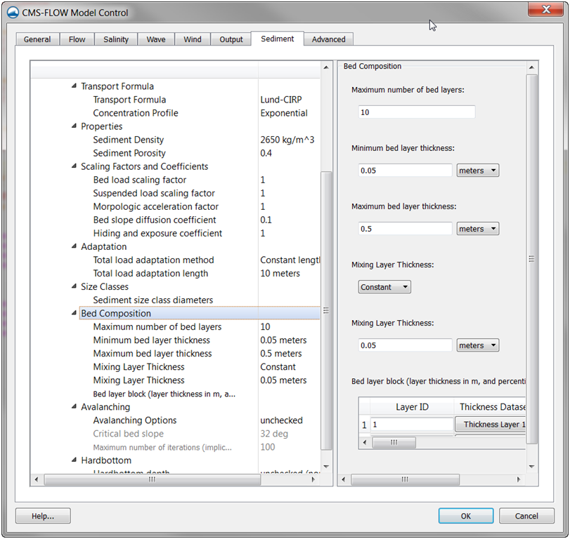
The basic bed layer settings are specified in the Bed Composition section of the Sediment tab in the CMS-Flow Model Control window (see figure below). The basic parameters for the bed layers are the maximum number of bed layers, and the minimum and maximum bed layer thicknesses.

Figure 2-88. Bed Composition section within the Sediment tab of the CMS-Flow Model Control window.

The CMS-Flow cards used to specify the maximum number of bed layers, and the minimum and maximum bed layer thickness are described in the table below.

Table 2-87. CMS card used to specify the total-load adaptation coefficient.

Input	Format	Notes
Maximum Number of Bed Layers	[cards=BED_LAYERS_MAX_NUMBER] [name=BedLayMaxNum, type=int, default=10, range=(5<BedLayMaxNum<20)]	The input number of bed layers must be less or equal to the maximum number of bed layers
Minimum Bed Layer Thickness	[cards=BED_LAYERS_MIN_THICKNESS] [name=BedLayMinThick, type=real, default=0.05, required=false, typical=(0.001<BedLayMinThick<0.2)] [name=BedLayMinThickUnits, type=char, optional=true, options=DistUnits, default=’m’]	Specifies the minimum bed layer thickness for all layers during the simulation.
Maximum Bed Layer Thickness	[cards=BED_LAYERS_MAX_THICKNESS] [name=BedLayMaxThick, type=real, default=0.5, required=false, typical=(0.1<BedLayMaxThick<1.0)] [name=BedLayMaxThicknits, type=char, optional=true, options=DistUnits, default=’m’ ]	Specifies the minimum bed layer thickness for all layers during the simulation.

Mixing Layer Thickness

The mixing layer is the first layer from the surface which is allowed to ex-change (or mix) sediments with the sediment transport. The mixing layer thickness is calculated based on the median grain size and bed form size. The option is also available to set the mixing layer to a constant. The CMS-Flow cards used for setting the mixing layer thickness to a constant is described in the table below.

Table 2-88. CMS-Flow used for setting a constant mixing layer thickness.

Input	Format	Notes
Mixing Layer Formulation	[cards=MIXING_LAYER_FORMULATION] [name=MixLayForm, type=char, default=CONSTANT options=(CONSTANT,AUTOMATIC)]	The input number of bed layers must be less or equal to the maximum number of bed layers
Mixing Layer Constant Thickness	[cards=MIXING_LAYER_THICKNESS_CONSTANT] [name=MixLayConst, type=real, default=0.05, required=false, typical=(0.001<MixLayConst<0.2)] [name=MixLayConstUnits, type=char, optional=true, options=DistUnits, default=’m’]	Sets the mixing layer thickness to a constant in meters.

=Notes=:

• Using a larger mixing layer will slow down the temporal change in bed material composition and enhance model stability, but will re-duce the accuracy of the bed composition estimates.

• Erosional cases tend to have smaller mixing layer thicknesses and depositional cases tend to have larger mixing layer thicknesses.

• The mixing layer thickness should NOT be used as a calibration parameter.

Bed Layer Thickness and Composition

The initial bed layer thickness and composition are specified at least one layer for the whole grid. The Layer ID corresponds to the layer number from the surface downwards. If the Layer ID is not specified in the card file, then it is assumed to be equal to the bed layer block sequential num-ber. In order to avoid having to specify all of the bed layers, the bed layer ID’s are allowed to have gaps in which case the missing bed layers or cop-ied from the first specified bed layer above. For example if bed layers 1 and 3 are specified and there is a maximum of 10 layers, then bed layer 2 is copied from bed layer 1, and bed layers 4 through 10 are copied from bed layer 3.

The bed composition is specified using percentile diameters which indicate the percentage of diameters smaller than a specific diameter. The percentile diameters are denoted by ,d_per where the subscript per indicates the percentage of diameters smaller than d.

=Notes=:

• There are several advantages to using percentile diameter datasets instead of the fraction of each sediment size class. The percentile diameters are independent of the sediment size classes and there-fore do not need to be changed if the size classes are changed. In addition the percentile diameters are easier to manipulate spatially than sediment fractions because the sum of the later must equal to one.

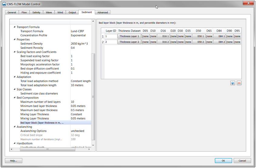
Figure 2-89. Bed layer block section within the Sediment tab of the CMS-Flow Model Control window in SMS 11.1.

A bed layer thickness and composition is defined with a bed layer block. The cards used to define the beginning and end of a bed layer block are described in the table below.

Table 2-89. CMS-Flow cards used to specify a Bed Layer block.

Input

Format

Notes

Begins a sediment size class block

[begin=BED_LAYER_BEGIN,

  block=BedLay, children=BedLayNum]

Begins a bed layer block.

Bed layer

number

[card=(LAYER,LAYER_NUMBER)]

[name=BedLayNum, type=float, default=none,

  range=(diam >0.06 ’mm’)]

[name=SedDens, type=char,

  options=DensUnits), default=’mm’]

Specifies the bed layer number from the surface. If not specified then set the sequential bed layer block number.

Ends a sediment size class block

[end=BED_LAYER_END, block=BedLay]

Ends a bed layer block

]

There are two methods for specifying each bed layer thickness:

1. Constant value

2. Spatially variable (dataset)

The CMS-Flow cards related to the bed layer thickness are described in the table below.

Table 2-90. CMS card used to specify the bed layer thickness

Input	Format	Notes
Bed layer thickness dataset	[cards=THICKNESS_DATASET, SMS_ver=(>11.1), CMS_ver=(>4.10.00)] [name=BedLayThickDatFile, type=char, example= "Flow_grid.h5"] [name=BedLayThickDatPath, type=char, example= "Flow/Datasets/D50 2"]	Specifies the file name and dataset path (within the file) for the bed layer thickness dataset.
Bed layer thickness value	[cards=THICKNESS_VALUE] [name=BedLayThickVal, type=real] [name=BedLayThickValUnits, type=char, optional=true, options=DistUnits, default=’m’ ]	Specifies the bed layer thickness as a constant value. .

There are four methods for specifying the bed layer composition:

1. D16, D50, and D84 Datasets

2. D35, D50, D90 Datasets

3. Cumulative Grain Size Distribution

The first two options assume a log-normal grain size distribution

\rho _{k}={\frac {\Delta d_{k}}{d_{k}\ ln\ \sigma _{g}{\sqrt {2\pi }}}}exp\left[-{\frac {1}{2}}\left({\frac {ln\ d_{k}-\ ln\ d_{g}}{ln\ \sigma _{g}}}\right)^{2}\right]

(2-33)

where $\rho _{k}$ is the fraction, $\Delta d_{k}=d_{uk}-d_{lk}$ is the size class bin width, $d_{k}$ is the size class diameter, and $d_{50}$ is the median grain size. The geometric standard deviation $\sigma _{g}$ can be defined using the method of moments

\sigma _{g}=exp{\sqrt {\Sigma \rho _{k}(ln\ d_{k}-ln\ d_{g})^{2}}}

(2-34)

It is noted that the geometric standard deviation is dimensionless.

The geometric mean d_g is in given by

d_{g}=exp\left(\Sigma \rho _{k}ln\ d_{k}\right)

(2-35)

An alternate approach to the above equation for obtaining geometric standard deviation is by using the graphical measures (cumulative percentile values) (Folk and Ward 1957)

\sigma _{g}\approx _{G}=exp\left({\frac {ln\ d_{16}-ln\ d_{84}}{4}}+{\frac {ln\ d_{5}-ln\ d_{95}}{6.6}}\right)

(2-36)

where $\sigma _{G}$ is a graphical measure of the geometric standard deviation.

Sediments with a geometric standard deviation $\sigma _{f}$ close to one are classified as well sorted and poorly graded (see table below).

Table 2-91. Sediment sorting classification based on the geometric standard deviation (Folk and Ward, 1957).

Geometric Standard Deviation	Sorting Classification
<1.27	Very well sorted
1.27-1.41	Well sorted
1.41-1.62	Moderately well sorted
1.62-2.00	Moderately sorted
2.00-4.00	Poorly sorted
4.00-16.00	Very poorly sorted
>16.00	Extremely poorly sorted

=Recommendations=:

• Areas with sediments with

\sigma _{g}

greater then approximate 1.41 should be simulated with multiple grain sizes.

D16, D50, and D84 Datasets

In this option, 2DH spatial datasets for the diameters corresponding to the 16^th, 50^th, and 84^th percentiles are specified for the whole computational domain. The bed composition is calculated using the log-normal distribution (Equation 2.28) with $d_{g}\approx d_{50}$ and

\sigma _{g}\approx \left({\frac {d_{84}}{d_{16}}}\right)^{1/2}

(2-37)

where the subscript indicates the percentile of the grain size diameter.

D30, D50, and D90 Datasets

In this option, 2DH spatial datasets for the diameters corresponding to the 30^th, 50^th, and 90^th percentiles are specified for the whole computational domain. The bed composition is calculated using the log-normal distribution (Equation 2.28)with $d_{g}\approx d_{50}$ and

\sigma _{g}\approx \left({\frac {d_{90}}{d_{35}}}\right)^{0.61}

(2-38)

where the subscript indicates the percentile of the grain size diameter.

Cumulative Grain Size Distribution

This option should be used in cases where the initial bed grain size distri-bution does not follow a log-normal distribution such as the case of a bi-modal distribution. In this option more than 3 percentile diameter da-tasets need to be specified with at least one below and above the 5o^th percentile. Currently the percentile diameters which are allowed in SMS 11.1 are: 5, 10, 16, 20, 30, 50, 64, 84, 90, and 95. The cumulative grain size distribution is linearly interpolated from the percentile diameters at the size class bounds and then converted to sediment fractions.

The CMS-Flow cards used to specify the bed composition are described in the table below

Table 2-92. CMS card used to specify the bed layer percentile diameters.

Input	Format
5th percentile diameter dataset	[cards=D05_DATASET, parent=BedLay] [name=d05file, type=char, example= "Flow_grid.h5"] [name=d05path, type=char, example= "Flow/Datasets/D05 1"]
10th percentile diameter dataset	[cards=D10_DATASET, parent=BedLay] [name=d10file, type=char, example= "Flow_grid.h5"] [name=d10path, type=char, example= "Flow/Datasets/D10 2"]
16th percentile diameter dataset	[cards=D16_DATASET, parent=BedLay] [name=d16file, type=char, example= "Flow_grid.h5"] [name=d16path, type=char, example= "Flow/Datasets/D16 3"]
20th percentile diameter dataset	[cards=D20_DATASET, parent=BedLay] [name=d20file, type=char, example= "Flow_grid.h5"] [name=d20path, type=char, example= "Flow/Datasets/D20 1"]
30th percentile diameter dataset	[cards=D30_DATASET, parent=BedLay] [name=d30file, type=char, example= "Flow_grid.h5"] [name=d30path, type=char, example= "Flow/Datasets/D30 1"]
50th percentile diameter dataset	[cards=D50_DATASET, parent=BedLay] [name=d50file, type=char, example= "Flow_grid.h5"] [name=d50path, type=char, example= "Flow/Datasets/D50 2"]
65th percentile diameter dataset	[cards=D64_DATASET, parent=BedLay] [name=d64file, type=char, example= "Flow_grid.h5"] [name=d64path, type=char, example= "Flow/Datasets/D65 2"]
84th percentile diameter datset	[cards=D84_DATASET, parent=BedLay] [name=d30file, type=char, example= "Flow_grid.h5"] [name=d84path, type=char, example= "Flow/Datasets/D84 3"]
90th percentile diameter dataset	[cards=D90_DATASET, parent=BedLay] [name=d90file, type=char, example= "Flow_grid.h5"] [name=d90path, type=char, example= "Flow/Datasets/D90 2"]
95th percentile diameter dataset	[cards=D95_DATASET, parent=BedLay] [name=d95file, type=char, example= "Flow_grid.h5"] [name=d95path, type=char, example= "Flow/Datasets/D95 1"]

=Notes=:

• When creating a percentile diameter dataset in SMS 11.1, the block number is appended to the end of the dataset name as for example “D50 2”. The number is used to distinguish datasets from different bed layer blocks and is not necessarily the same as the bed layer ID number.

• If the percentile diameters are specified outside of a bed layer block, then they are assumed to belong to the first and only layer.

Advanced Bed Layer Composition

Two additional options are available for specifying the bed composition:

1. D50 dataset and constant geometric standard deviation

2. Size class fractions

A description of the CMS-flow card used to select each bed material com-position option is described in the table below.

Table 2-93. CMS-Flow card used to specify the option for specifying the bed material composition.

Input	Format
Bed Layer Geometric Standard Deviation	[cards=(SIGMA,GEO_STD_DEV), parent=BedLay, SMS_ver=none, CMS_ver=(>4.10.00)] [name=BedLaySig, type=real, range=(BedLaySig>=1.0), default=1.5]
Bed Layer Size Class Fractions	[cards=FRACTIONS, parent=BedLay, SMS_ver=none, CMS_ver=(>4.10.00)] [name=SedClassNum, type=int] for(k=1:SedClassNum, [name=BedLayFrac(k), type=real, range=(0.0>BedLayFrac(k)<1.0)])

=Notes=:

• The above two options are not available in SMS and are therefore considered advanced.

• The geometric standard deviation must always be equal or larger than 1.0.

• When the user specifies the sediment fractions, the sum of the fractions must equal 1.0. If they do not equal 1.0, the fractions are divided by the sum so that they equal 1.0.

Examples

In the case of single-sized sediment transport, the option is available to specify a median grain size dataset which is used to calculate a hiding and exposure correction to the single transport grain size.

Example 2-87. Bed composition specification for a single-sized sediment transport simulation.

example 2-88

Hiding and Exposure

The hiding and exposure is an important parameter for sediment transport. Currently, there are no well established coastal sediment transport formulas for nonuniform sediments. The most common ap-proach is to adapt single-size transport formulas by applying correction factors. The most common of these factors is the hiding and exposure correction. The implementation of this factor varies depending on the transport formula and usually involves a coefficient (exponent) which needs to be calibrated. Because all of the transport formulas used in CMS were originally developed for uniform sediments, there is still a large un-certainty in the value of the hiding and exposure coefficient. It is expected that the hiding and exposure coefficient will be different for different transport formula especially since the implementation of the hiding and exposure correction may be different for different formula.

Single-sized Sediment Transport

For single-sized sediment transport, the correction function for hiding and exposure is calculated following Parker et al. (1982) as

\xi _{k}=\left({\frac {d_{50}}{d_{k}}}\right)^{m}

(2-39)

where m is the hiding and exposure coefficient. The approach has been successfully applied to Shinnecock Inlet, NY to simulate morphology change at a coastal inlet (Sánchez and Wu 2011a). If the sediment is not well sorted, then a multiple sediment fractions need to be simulated (see section below)

Multiple-sized Sediment Transport

The hiding and exposure of the each sediment size class is considered by modifying the critical shields parameter $\Theta _{ck}$ for each sediment size class based on Wu et al. (2000)

\xi _{k}=\left({\frac {P_{ek}}{P_{hk}}}\right)^{-m}

(2-40)

where m is an empirical coefficient that varies for each transport formula, approximately equal to 0.6-1.0. P_ek and P_hk are the total hiding and exposure probabilities and are calculated as

P_{hk}=\sum _{j=1}^{N}p_{1j}{\frac {d_{j}}{d_{k}+d_{j}}}\quad \quad P_{ek}=\sum _{j=1}^{N}p_{1j}{\frac {d_{k}}{d_{k}+d_{j}}}

(2-41)

where N is the number of grain size classes.

The hiding and exposure coefficient used for both the single- and multiple-sized sediment transport is specified with the same CMS-Flow card (see table below).

table 2-94

=Recommendations=:

• Due to the uncertainty in the hiding and exposure correction coeffi-cient. It is recommended to always calibrate the hiding and exposure coefficient. If no or limited data is available for calibration then a sensitivity analysis should be done

=Note=:

• The hiding an exposure coefficient may have a different “best” value for different transport formula.

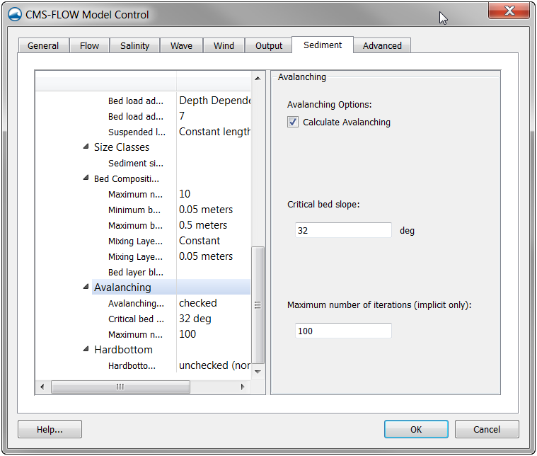
Avalanching

Avalanching is the process of sediment sliding when the critical angle of repose is reached. In CMS, avalanching is simulated using a mass con-servative relaxation method which limits the bed slope to the critical angle of repose. For most coastal applications, the critical angle of repose is never reached, so it is not needed. The CMS-Flow cards used for specifying avalanching, and its options, are described in table below.

Figure 2-90. Avalanching section within the Sediment tab of the CMS-Flow Boundary Conditions window.

The table below describes the CMS-Flow cards used to specify the ava-lanching options.

table 2-95

example 2-89

=Notes=:

• Turning on avalanching increases slightly the computational time.

• For most coastal morphodynamic applications, the avalanching can be turned off since the angle of repose is almost never reached. If a simulation is run without avalanching and steep angles are found in the calculated morphology change, then the simulation should be rerun with avalanching turned on.

User Guide 012

Contents

Total-Load Correction Factor

Bed Composition

Single-sized Sediment Transport

Multiple-sized Sediments

D16, D50, and D84 Datasets

D30, D50, and D90 Datasets

Cumulative Grain Size Distribution

Advanced Bed Layer Composition

Examples

Hiding and Exposure

Single-sized Sediment Transport

Multiple-sized Sediment Transport

Avalanching

Navigation menu

User Guide 012

Total-Load Correction Factor

Bed Composition

Single-sized Sediment Transport

Multiple-sized Sediments

D16, D50, and D84 Datasets

D30, D50, and D90 Datasets

Cumulative Grain Size Distribution

Advanced Bed Layer Composition

Examples

Hiding and Exposure

Single-sized Sediment Transport

Multiple-sized Sediment Transport

Avalanching

Navigation menu

Search