User Guide 013

Hard Bottom

Hard Bottom is a morphologic constraint that provides the capability to simulate mixed bottom types within a single simulation. This cell-specific feature limits the erodability of the constrained cells down to a specified depth below the water surface. During sediment transport calculations, exposed hard bottom cells may become covered through deposition. By default, CMS-Flow cells are fully-erodible cells with no specified hard bottom depth (inactive cells; denoted by the CMS-Flow null value of -999.0). Hard bottom only needs to be specified only for computational (ocean) cells.

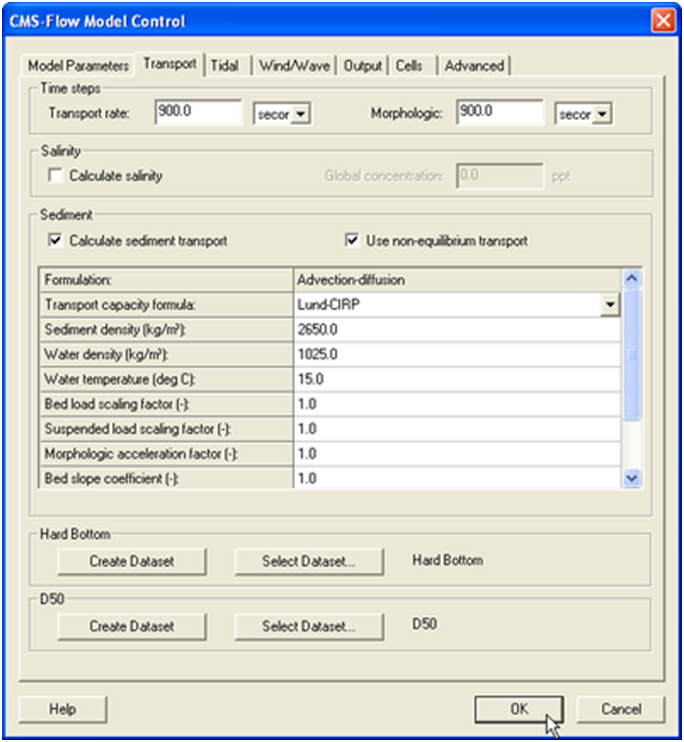
Figure 2 91. CMS-Flow Model Control window showing the location where the hard bottom dataset is specified.

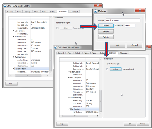
Figure 2 92. Specification of the Hardbottom Dataset in the Sediment tab of the CMS-Flow Model Control window in SMS 11.1.

Within the CMS-Flow Model Control window, the hard bottom dataset can be created from the Sediment tab. If the dataset does not exist, it can be created using the Create Dataset button. If a dataset exists (created using the Data Calculator) which represents the intended hard bottom specifications, the Select Dataset button can be used to select such dataset and copy the values to the hard bottom dataset.

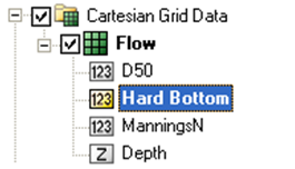
When specified, cell hard bottom depths will appear in the Project Explorer as a scalar dataset beneath the CMS-Flow grid. This dataset cannot be deleted, though it can be edited like any other dataset. A CMS-Flow simulation must contain the hard bottom dataset (even if it is not specified) so SMS will create a defaulted (inactive cells) dataset if it does not already exist when saving the simulation. The hard bottom dataset can created, edited, viewed and verified using the following SMS interface features.

example 2-90

Boundary and Initial Conditions

In the case of the Equilibrium Total Load sediment transport model, all boundaries are set to the equilibrium transport rate. For the Equilibrium Bed Load plus Advection Diffusion model, the suspended load is specified as the equilibrium concentration at inflow cells and a zero gradient at outflow cells. For the Total load nonequilibrium sediment transport model, the sediment concentration is set to the equilibrium concentration at inflow cells and a zero gradient boundary condition is applied at outflow cells.

In the case an initial conditions file is NOT specified both the hydrody-namics and sediment concentrations are initialized as zero. If an initial conditions file is specified, than the initial sediment concentrations are read in. If an initial conditions file is specified but without the sediment concentration, than the initial sediment concentration is set to the equilibrium concentration.

table 2-96

Step-by-Step Sediment Transport Application for Shark River Inlet, NJ TBC

Numerical Methods

Temporal Solution Scheme

This refers to the temporal discretization of the hydrodynamic, sediment and salinity transport equations. There are two options in CMS: Implicit and Explicit. The implicit scheme uses a time step on the order of 5-20 minutes and is designed for tidal flow, and mid-term morphology change. The explicit scheme uses a time step on the order of 0.5-1.0 seconds and is appropriate for cases that vary quickly in time such as flooding or barrier island breaching.

table 2-97

Note:

• The second order implicit temporal scheme requires three time step levels. Therefore, for the first time step, the model uses the first order two-level temporal scheme. In addition, if the time step is increased or decreased during the simulation. The first order scheme is used.

Implicit Solver Options

The solvers implemented in the implicit temporal solution scheme are the SIP, ICCG, Gauss-Seidel, Gauss-Seidel with Successive-Over-Relaxation, BICGSTAB, and GMRES. Currently, the same solver is applied to flow, sediment and salinity. The default solver is the GMRES. The solver may be changed using the advanced card in the table below. The SIP and ICCG solvers are only available for non-telescoping grids. The maximum number of outer and inner loop iterations may also be changed. The outer loop is the loop over which the governing equations are solved successively, while the inner loop is the loop within the matrix solver for each governing equation.

table 2-98

Skewness Correction

When the lines connecting cell centers do not intercept the cell-face centers, the cells are said to be skewed. When interpolating variables to the cell-face or calculating cell-face gradients a correction is needed for second order accuracy. There are several ways in which the correction can but involves some form of reconstruction of the variable on the cell face or within the neighboring cells. In CMS a linear cell reconstruction is performed within skewed cells for the correction.

table 2-99

Advection Schemes

As in the case of the implicit solution scheme, the same advection scheme is applied for the flow, sediment and salinity transport equations. Future versions of the CMS will allow the user to select different advection schemes for different governing equations. There are several choices for advection schemes with the implicit model which are listed in the table below. The schemes range from first to third order. The hybrid scheme is fast but is the most diffusive. The exponential scheme is based on the 1D analytical solution to a steady-state advection-diffusion equation and produces very stable results. The HLPA is very stable and non-diffusive, but requires slightly more computational time. For most applications, the exponential scheme is recommended and is set as the default. The advection scheme may be change using the advanced card described in the table below.

table 2-100

Wetting and Drying

In CMS, a minimum depth is required for cells to be considered. A cell is classified as wet if the total water depth is larger than this depth. Cell faces are either classified as either open if the two cells neighboring cells are wet or otherwise closed (i.e. cell faces are not classified as wet or dry) , in order to improve stability.

table 2-101

Parallelization

The CMS-Flow is parallelized for PC’s with multi-core processors using OpenMP. The parallelization works by splitting the computational work into “threads” among several cores. Some cores are hyper-threaded, meaning a single core may support two threads. The number of threads is specified in the CMS-Flow Model Control Window. The number of threads must be equal or greater to 1 and cannot be larger than the number of threads available on the machine. If a number is specified which is larger than the maximum number available on the machine, then the code will default to the maximum number available.

table 2-102

Note:

• The OpenMP parallelization requires that compatibility OpenMP run-time library (libiomp5md.dll) be in search paths.

• When running multiple simulations at once, the user should keep track of how many threads are being used by each simulation and make sure that the maximum number of threads on the computer is not exceeded. Exceeding the maximum number of threads on the computer will slow down the simulations and also make the computer slow.

• It is always recommended to at least leave one thread unused by model simulations so that the computer is responsive while the simulations are running.

Hot Start

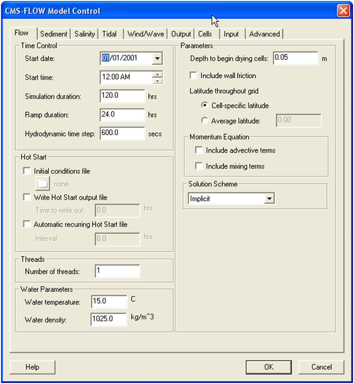
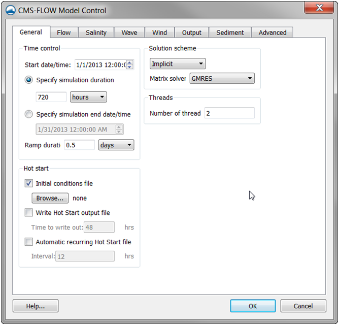
The term “hot start” refers to starting a simulation with an initial condition other zero (cold start). Hot starts are used for specifying initial conditions other than the default zero value or restarting simulations at intermediate times. The hot start controls are set in the CMS-Flow Model Control window under the Flow tab in SMS 11.0 (see Figure 2-94) and in the General tab in SMS 11.1 and later (see Figure 2 95).

Figure 2-94. Location of Hot Start input and output options within the Flow tab of the CMS-Flow Model Control window in SMS 11.0.

The hot start options are the input Initial Conditions file, the output time and recurring interval for the Hot Start file. A description of these controls and options are provided in the subsequent sections.

Hot Start Output File The CMS Hot Start feature lets the user restart simulations that have been ended or stopped due to for example electric outages, hardware malfunctions, or model crashes. In the case of a model crash the user, may restart the model using larger solver iterations and/or time steps to stabilize the simulation. The user has the option to specify a hot start output time or an interval for outputting a recurring hot start file. Every time the hot start file is written, it overwrites the previous information. The CMS Hot Start file saves information on the water elevation (pressure), and current velocities. If the sediment transport is active, the water depth and sediment concentrations are also saved for each size class. The CMS Hot Start File is a binary XMDF file, has the name Hot_Start.h5 and is saved in the directory of the CMS-Flow files. Figure 2 96 shows the structure of the hot start file. After saving a CMS Hot Start File, it is a good idea to rename the file with a different name before using it as an initial conditions file. This way, the file will not be overwritten in future simulations.

figure 2-96

table 2-103

Input	Format	Notes
Hot start output file	[cards=HOT_START_OUTPUT_FILE, versions=(>3.75.00)] [name=HotStartFile, type=char, default=”Hot_Start.h5”, optional=true]	Specifies the name of the hot start output file

example 2-91

example 2-92

table 2-104

Initial Conditions Input File There are several situations where it is convenient to specify a user defined initial condition (hot start) file. For example, if the user forgets to setup the model output a hot start file or when running idealized cases with known initial conditions. A hot start file can easily be created and exported by the user from the SMS interface. The model requires at water levels, current velocities, concentrations, and water depths. Any datasets that are missing from the initial file are assigned a default value which depends on the dataset. If the water level or current velocities are not specified, they are set to zero. If the depth is not specified, then it is set to the input grid depth. If the sediment concentrations are not specified, then they are set to the equilibrium concentrations. It is important to note that the names and paths of the initial condition datasets are important.

table 2-105

The initial conditions file contains grid datasets with initial values for water levels, current velocities, salinity and sediment concentrations, bed composition, bed layer thicknesses, and water depth. All of the input da-tasets are optional. If the dataset does not exist than it is set to the default value.

table 2-106

example 2-93

example 2-94

example 2-95

Note: • The time of the initial conditions file is with respect to a reference time of the current simulation. The default units is hours but may be changed to any units. • The initial condition and hot start files only contain a single time step. Therefore, when selecting the second-order backward difference im-plicit scheme which uses two previous time steps, the first time step is calculated using the first-order backward difference scheme. In the case of the explicit temporal scheme, only the first-order forward dif-ference scheme is available.

Creating an Initial Conditions File The steps for creating a user defined hot start or initial condition file from a CMS-Flow solution file are outlined below. 1. Import CMS-Flow grid and solution file. 2. Sample a time step of the solution datasets for use in the initial condi-tion 2.1. Click on Data | Data Calculator 2.1.1. Under the Tools section, select Sample time steps. 2.1.2. Under the Datasets section, click on the Water Elevation 3. Export the initial condition datasets to an XMDF file

figure 2-97

figure 2-98

table 2-107

Output Options Global Output Global output refers to the variables that are output on every active cell on the grid. The global output options are specified in Output tab of the CMS-Flow Model Control window. More information on the global output variables, groups and CMS-Flow cards is provided in the sections below.

figure 2-99

Output Datasets Global output datasets are divided into groups and each group is assigned an output times, and file. A description of the various output datasets and the associated groups is provided in the table below.

table 2-108

Output Time Series and Lists The times at which each group is output is determined by the selecting one of four user defined output time series or lists. In SMS versions 10.1 and earlier, the output time series were used. However, because the output time series can become very large for long-term simulations, the time series have been replaced by lists in which the output times are specifying a list of starting, ending and increments. This option is more compact and also makes it easier to manually change the output options in the cmcards file.

table 2-109