JALBTCX/QRStep4: Difference between revisions
(Created page with "{{DISPLAYTITLE:Quick Response Toolbox: Step 4 - Volume by Zonal Statistics}} File:QR Step4.jpg|thumb|right|alt=A screenshot of the ArcPro geoprocessing panel for Step 4. The "Difference Grid" input allows the user to select the file from a dropdown menu or the file explorer. The "Before Raster Date" and "After Raster Date" inputs are text boxes which require the input be Year, Month, then Date with no spaces or punctuation (YYYYMMDD). The "Vertical Unit of Input Raster...") |
mNo edit summary |
||
| (2 intermediate revisions by the same user not shown) | |||
| Line 4: | Line 4: | ||
'''Summary:''' This step uses raster math to create a “Difference Grid”. First, elevation surfaces are created for each year of data using the clip mask. The script then uses arcpy.sa.Minus to get the difference grid between two input rasters. The output raster cell size is determined by default based on the cell size of the input raster with the smallest cells. For example, if a DEM raster with a 1m resolution is subtracted by a DEM raster with a 3m resolution, the output will be a 1m raster. The outputs of this step include surface grids and a difference grid to be used in subsequent steps for volume change. | '''Summary:''' This step uses raster math to create a “Difference Grid”. First, elevation surfaces are created for each year of data using the clip mask. The script then uses arcpy.sa.Minus to get the difference grid between two input rasters. The output raster cell size is determined by default based on the cell size of the input raster with the smallest cells. For example, if a DEM raster with a 1m resolution is subtracted by a DEM raster with a 3m resolution, the output will be a 1m raster. The outputs of this step include surface grids and a difference grid to be used in subsequent steps for volume change. | ||
'''Difference Grid:''' The difference grid created in Step 3 | '''Difference Grid:''' The difference grid created in [[JALBTCX/QRStep3|Step 3]]. | ||
'''Before Raster Date (YYYYMMDD):''' Desired label for the before raster. The year is suggested but the user is free to decide. | '''Before Raster Date (YYYYMMDD):''' Desired label for the before raster. The year is suggested but the user is free to decide. | ||
| Line 10: | Line 10: | ||
'''After Raster Date (YYYYMMDD):''' Desired label for the after raster. The year is suggested but the user is free to decide. | '''After Raster Date (YYYYMMDD):''' Desired label for the after raster. The year is suggested but the user is free to decide. | ||
''' Vertical Unit of Input Raster:''' | ''' Vertical Unit of Input Raster:''' The vertical unit of the raster, options include meters or feet. | ||
'''Transect Mask:''' Transect mask created in Step 2. | '''Transect Mask:''' Transect mask created in [[JALBTCX/QRStep2|Step 2]]. | ||
''' Volume Unit:''' | ''' Volume Unit:''' Desired unit for volume calculation, options include cubic yards, cubic meters or cubic feet. | ||
'''Output Geodatabase:''' Full file path, including name and file extension, for desired output geodatabase. | '''Output Geodatabase:''' Full file path, including name and file extension, for desired output geodatabase. | ||
| Line 24: | Line 24: | ||
Figure 7 below displays the difference volume output for the Homer, AK example data. When the output from this step is loaded into the map the user will have to alter the symbology. Below the data is symbolized based on the “dVol” attribute. | Figure 7 below displays the difference volume output for the Homer, AK example data. When the output from this step is loaded into the map the user will have to alter the symbology. Below the data is symbolized based on the “dVol” attribute. | ||
[[File:QRFigure7.jpg|thumb|center|alt=A view of the difference volume polygons visualized by volume change in cubic meters. The bins show blue for accretion and red for erosion There is one for the whole project as well as a zoomed in extent. This coastline contains small areas of high magnitudes of erosion with large areas of low magnitude accretion.|Figure 7: Difference volume output from Step 4 at Homer, AK. The bottom figure (b) displays the zoomed area outlined in yellow from (a) to show individual bins.]] | [[File:QRFigure7.jpg|thumb|center|alt=A view of the difference volume polygons visualized by volume change in cubic meters. The bins show blue for accretion and red for erosion There is one for the whole project as well as a zoomed in extent. This coastline contains small areas of high magnitudes of erosion with large areas of low magnitude accretion.|Figure 7: Difference volume output from Step 4 at Homer, AK. The bottom figure (b) displays the zoomed area outlined in yellow from (a) to show individual bins.|475x475px]] | ||
==Useful Links== | ==Useful Links== | ||
[[JALBTCX|JALBTCX Main Documentation Page]] | [[JALBTCX|JALBTCX Main Documentation Page]] | ||
[[JALBTCX/QRReferences|Refences: Quick Response Toolbox]] | [[JALBTCX/QRReferences|Refences: Quick Response Toolbox]] | ||
Latest revision as of 21:27, 11 December 2024
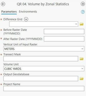
Summary: This step uses raster math to create a “Difference Grid”. First, elevation surfaces are created for each year of data using the clip mask. The script then uses arcpy.sa.Minus to get the difference grid between two input rasters. The output raster cell size is determined by default based on the cell size of the input raster with the smallest cells. For example, if a DEM raster with a 1m resolution is subtracted by a DEM raster with a 3m resolution, the output will be a 1m raster. The outputs of this step include surface grids and a difference grid to be used in subsequent steps for volume change.
Difference Grid: The difference grid created in Step 3.
Before Raster Date (YYYYMMDD): Desired label for the before raster. The year is suggested but the user is free to decide.
After Raster Date (YYYYMMDD): Desired label for the after raster. The year is suggested but the user is free to decide.
Vertical Unit of Input Raster: The vertical unit of the raster, options include meters or feet.
Transect Mask: Transect mask created in Step 2.
Volume Unit: Desired unit for volume calculation, options include cubic yards, cubic meters or cubic feet.
Output Geodatabase: Full file path, including name and file extension, for desired output geodatabase.
Project Name (must start with letters): Desired name for the project. The output file name will be “User-defined project name” + “_’Type of Grid’_” + “before year” + “after year”. This tool will output: one before raster grid per segment, one after raster per segment and one difference grid per segment.
Best Practices & Example Data:
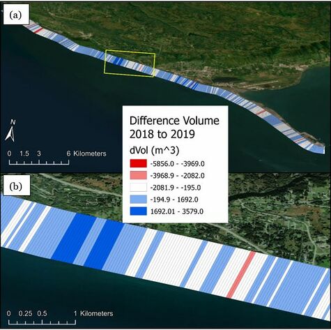
Figure 7 below displays the difference volume output for the Homer, AK example data. When the output from this step is loaded into the map the user will have to alter the symbology. Below the data is symbolized based on the “dVol” attribute.

