CMS-Flow Model Parameters: Difference between revisions
| (80 intermediate revisions by 2 users not shown) | |||
| Line 21: | Line 21: | ||
===Hot Start=== | ===Hot Start=== | ||
[[File:CMSFlow Model Parameters GeneralTab Hotstart V13.2.12.png|500px|thumb| | [[File:CMSFlow Model Parameters GeneralTab Hotstart V13.2.12.png|500px|thumb|center|Figure 3: Hot start parameters on CMS-Flow Model Control]] | ||
The term Hot start (Figure 3) refers to starting a simulation with an initial condition other zero (cold start). Hot starts are used for specifying initial conditions or restarting simulations at intermediate times. The hot start controls are set in the ''Flow'' tab of the ''CMS-Flow Model Control'' window. | The term Hot start (Figure 3) refers to starting a simulation with an initial condition other zero (cold start). Hot starts are used for specifying initial conditions or restarting simulations at intermediate times. The hot start controls are set in the ''Flow'' tab of the ''CMS-Flow Model Control'' window. | ||
Hot Start | ====Hot Start File==== | ||
[[Image:Hot_Start_HDFView.png|thumb|right|500px| Figure 4. HDFView showing the structure of the CMS Hot Start File. ]] | [[Image:Hot_Start_HDFView.png|thumb|right|500px| Figure 4. HDFView showing the structure of the CMS Hot Start File. ]] | ||
The CMS hot start feature CMS lets the user restart simulations that have been stopped due to electric outages, hardware malfunctions, or model crashes. In the case of a model crash the user, may restart the model using larger solver iterations and/or time steps to stabilize the simulation. The user has the option to specify a hot start output time or an interval for outputting a recurring hot start file. Every time the hot start file is written, it overwrites the previous information. The CMS Hot Start file saves information on the water elevation (pressure), and current velocities. If the sediment transport is active, then the water depth and sediment concentrations are also saved for each size class. Only the very last record of information is preserved (no starting from earlier intervals). | The CMS hot start feature CMS lets the user restart simulations that have been stopped due to electric outages, hardware malfunctions, or model crashes. In the case of a model crash the user, may restart the model using larger solver iterations and/or time steps to stabilize the simulation. The user has the option to specify a hot start output time or an interval for outputting a recurring hot start file. Every time the hot start file is written, it overwrites the previous information. The CMS Hot Start file saves information on the water elevation (pressure), and current velocities. If the sediment transport is active, then the water depth and sediment concentrations are also saved for each size class. Only the very last record of information is preserved (no starting from earlier intervals). | ||
| Line 42: | Line 42: | ||
| AUTO_HOT_START_INTERVAL || REAL || none || none || Sets the recurring hot start output interval . | | AUTO_HOT_START_INTERVAL || REAL || none || none || Sets the recurring hot start output interval . | ||
|} | |} | ||
====Initial conditions file==== | |||
[[File:CMSFlow Model Parameters GeneralTab Hotstart SavingCondFilesV13.2.12.png|300px|thumb|right|Figure 5 Dataset Toolbox showing a time step sample of the water elevation and current velocity datasets for use in a hot start (initial condition) file.]] | |||
[[File:CMSFlow Model Parameters GeneralTab Hotstart ExportingConditionsFilesV13.2.12.png|250px|thumb|Figure 6.a Dataset Toolbox showing a time step sample of the water elevation and current velocity datasets for use in a hot start (initial condition) file.]] | |||
[[File:CMSFlow Model Parameters GeneralTab Hotstart ExportingCondFilesV13.2.12.png|300px|thumb|Figure 6.b Saving conditions files]] | |||
There are several situations where it is convenient to specify a user defined initial condition (hot start) file. For example, if the user forgets to setup the model output a hot start file or when running idealized cases with known initial conditions. A hot start file can easily be created and exported by the user from the SMS interface. The model requires at water levels, current velocities, concentrations, and water depths. Any datasets that are missing from the initial file are assigned a default value which depends on the dataset. If the water level or current velocities are not specified, they are set to zero. If the depth is not specified, then it is set to the input grid depth. If the sediment concentrations are not specified, then they are set to the equilibrium concentrations. It is important to note that the names and paths of the initial condition datasets are important. | There are several situations where it is convenient to specify a user defined initial condition (hot start) file. For example, if the user forgets to setup the model output a hot start file or when running idealized cases with known initial conditions. A hot start file can easily be created and exported by the user from the SMS interface. The model requires at water levels, current velocities, concentrations, and water depths. Any datasets that are missing from the initial file are assigned a default value which depends on the dataset. If the water level or current velocities are not specified, they are set to zero. If the depth is not specified, then it is set to the input grid depth. If the sediment concentrations are not specified, then they are set to the equilibrium concentrations. It is important to note that the names and paths of the initial condition datasets are important. | ||
{| class=wikitable border="1" | {| class=wikitable border="1" | ||
! Variable !! Path and name | ! Variable !! Path and name | ||
|- | |- | ||
| Water surface elevation || Datasets\Water_Elevation | | Water surface elevation || Datasets\Water_Elevation | ||
| Line 55: | Line 58: | ||
| Salinity concentrations|| Datasets\Salinity | | Salinity concentrations|| Datasets\Salinity | ||
|} | |} | ||
Steps for creating a user defined hot start or initial condition file | Steps for creating a user defined hot start or initial condition file | ||
:1. Import CMS-Flow grid and solution file. | :1. Import CMS-Flow grid and solution file. | ||
:2. Sample a time step of the solution datasets for use in the initial condition | :2. Sample a time step of the solution datasets for use in the initial condition | ||
::*Click on Data | Data Calculator (Figure 5) | ::*Click on Data | Data Calculator (Figure 5) | ||
::*Under the Tools section, select Sample time steps. | ::*Under the Tools section, select Sample time steps. | ||
::*Under the Datasets section, click on the variable desired to be save (water surface elevation, current velocity, sediment concentrations or salinity concentrations) | ::*Under the Datasets section, click on the variable desired to be save (water surface elevation, current velocity, sediment concentrations or salinity concentrations) | ||
:3. Export the initial condition datasets to an XMDF file (Figure 6) | :3. Export the initial condition datasets to an XMDF file (Figure 6) | ||
*Write Hot Start output file [On/Off] | *Write Hot Start output file [On/Off] | ||
| Line 73: | Line 72: | ||
===Solution Scheme=== | ===Solution Scheme=== | ||
[[File:CMSFlow Model Parameters GeneralTab Flow SolutionScheme V13.2.12.png|500px|thumb| | [[File:CMSFlow Model Parameters GeneralTab Flow SolutionScheme V13.2.12.png|500px|thumb|center|Figure 7 Solution Scheme options]] | ||
This refers to the temporal discretization of the hydrodynamic, sediment and salinity transport equations. There are two options in CMS: implicit and explicit. | This refers to the temporal discretization of the hydrodynamic, sediment and salinity transport equations. There are two options in CMS: implicit and explicit. | ||
CMS-Flow has both implicit and explicit solution schemes. | |||
======[https://cirpwiki.info/wiki/CMS-Flow:Implicit Implicit]====== | |||
CMS-Flow implicit uses a generic Cartesian grid which can be regular, nouniform, or locally refined by splitting cells into two or four (only splitting into four supported by the interface at moment). Only three requirements are im-posed on the input grid: CMS-Flow Computational Grid | |||
**1. Cells must have a rectangular shape. Irregularly shaped cells are not allowed. | |||
**2. Cells may have a total of four to six neighboring cells (faces). | |||
**3. Only two cells are allowed in the same neighboring direction (i.e. North, South, East, West). | |||
======[https://cirpwiki.info/index.php?title=CMS-Flow:Explicit&action=edit&redlink=1 Explicit]====== | |||
The explicit solver is designed for dynamic problems with extensive wetting and drying which require small computational time steps, while the implicit solver is intended for simulating tidal and wave-induced circulation at tidal inlets, navigation channels, and adjacent beaches. A detailed description of the theoretical and numerical formulation of the explicit solver can be found in Buttolph et al. (2006) and is not repeated here. The sections below refer to the implicit solver. | |||
The influence of the sub-grid scale turbulence can be particularly relevant in these situations. The implicit hydrodynamic model is capable of handling subcritical, transcritical and supercritical flow regimes but may require a very small time for transcritical and super-critical flows making the computation making the model inefficient. | |||
For flows with a high Froude number, it is recommended to use the explicit flow model. Flow through structures is handled using empirical equations. | |||
=====[https://cirpwiki.info/wiki/CMSFlow_Matrix_Solver Matrix Solver]===== | =====[https://cirpwiki.info/wiki/CMSFlow_Matrix_Solver Matrix Solver]===== | ||
[[File:CMSFlow_Model_Parameters_GeneralTab_Matrix_Solver_V13.2.12.png|500px|thumb| | [[File:CMSFlow_Model_Parameters_GeneralTab_Matrix_Solver_V13.2.12.png|500px|thumb|center|Figure 8. Hot start parameters on CMS-Flow Model Control]] | ||
Matrix solver (Figure | Matrix solver (Figure 8): | ||
*[https://cirpwiki.info/wiki/CMSFlow_Matrix_Solver#Gauss- | *[https://cirpwiki.info/wiki/CMSFlow_Matrix_Solver#Gauss-Seidel Gauss-Seidel] | ||
*[https://cirpwiki.info/wiki/CMSFlow_Matrix_Solver#Gauss- | *[https://cirpwiki.info/wiki/CMSFlow_Matrix_Solver#Gauss-Seidel_SOR Gauss-Seidel-SOR] | ||
*[https://cirpwiki.info/wiki/CMSFlow_Matrix_Solver# | *[https://cirpwiki.info/wiki/CMSFlow_Matrix_Solver#BiCGStab BicGSTab] | ||
*[https://cirpwiki.info/wiki/CMSFlow_Matrix_Solver#GMRES GMRES] | *[https://cirpwiki.info/wiki/CMSFlow_Matrix_Solver#GMRES GMRES] | ||
===Threads=== | ===Threads=== | ||
[[File:CMSFlow Model Parameters GeneralTab Threads V13.2.12.png|500px|thumb| | [[File:CMSFlow Model Parameters GeneralTab Threads V13.2.12.png|500px|thumb|center|Figure 9. CMS Flow General Tab Threads Version 13.2.12]] | ||
*Number of threads (Figure 7) | *Number of threads (Figure 7) | ||
The CMS-Flow is parallelized for PC’s with multi-core processors using OpenMP. The parallelization works by splitting the computational work into “threads” among several cores. Some cores are hyper-threaded, meaning a single core may support two threads. The number of threads is specified in the CMS-Flow Model Control Window. The number of threads must be equal or greater to 1 and cannot be larger than the number of threads available on the machine. If a number is specified which is larger than the maximum number available on the machine, then the code will default to the maximum number available. | The CMS-Flow is parallelized for PC’s with multi-core processors using OpenMP. The number of threads used for parallel processing. The parallelization works by splitting the computational work into “threads” among several cores. Some cores are hyper-threaded, meaning a single core may support two threads. The number of threads is specified in the CMS-Flow Model Control Window. The number of threads must be equal or greater to 1 and cannot be larger than the number of threads available on the machine. If a number is specified which is larger than the maximum number available on the machine, then the code will default to the maximum number available. | ||
For more detail, see [https://cirpwiki.info/wiki/CMS-Flow:Multiple_Processor_Capability#Multiple_Processor_Capability Multi Processor Capability] | For more detail, see [https://cirpwiki.info/wiki/CMS-Flow:Multiple_Processor_Capability#Multiple_Processor_Capability Multi Processor Capability] | ||
| Line 121: | Line 112: | ||
=== Parameters === | === Parameters === | ||
[[File:CMSFlow Model Parameters GeneralTab Flow Parameters V13.2.12.png|500px|thumb| | [[File:CMSFlow Model Parameters GeneralTab Flow Parameters V13.2.12.png|500px|thumb|center| Figure 10. CMS Flow Parameters Version 13.2.12]] | ||
*Hydrodynamic Time Step | *Hydrodynamic Time Step | ||
*Wetting and drying* | *Wetting and drying* | ||
In the numerical simulation of the surface water flows with sloped beaches, sand bars and islands, the water edges change with time, with part of the nodes being possibly wet or dry. In the present model, a threshold flow depth (a small value such as 0.02 m in field cases) is used to judge drying and wetting. If the flow depth on a node is larger than the threshold value, this node is considered to be wet, and if the flow depth is lower than the threshold value, this node is dry. Because a fully implicit solver is used in the present model, all the wet and dry nodes participate in the solution. Dry nodes are assigned a zero velocity. On the water edges between the dry and wet nodes, the wall-function approach is applied. | In the numerical simulation (Figure 10) of the surface water flows with sloped beaches, sand bars and islands, the water edges change with time, with part of the nodes being possibly wet or dry. In the present model, a threshold flow depth (a small value such as 0.02 m in field cases) is used to judge drying and wetting. If the flow depth on a node is larger than the threshold value, this node is considered to be wet, and if the flow depth is lower than the threshold value, this node is dry. Because a fully implicit solver is used in the present model, all the wet and dry nodes participate in the solution. Dry nodes are assigned a zero velocity. On the water edges between the dry and wet nodes, the wall-function approach is applied. | ||
*Wave Fluxes and Roller Fluxes | *Wave Fluxes and Roller Fluxes | ||
| Line 136: | Line 127: | ||
=== Bottom and wall friction === | === Bottom and wall friction === | ||
In this section, users may specify wave current bottom friction and roughness dataset (Figure | In this section, users may specify wave current bottom friction and roughness dataset (Figure 11). | ||
[[File:CMSFlow Model Parameters GeneralTab Flow BottomandWallFrictionV13.2.12.png|500px|thumb| | [[File:CMSFlow Model Parameters GeneralTab Flow BottomandWallFrictionV13.2.12.png|500px|thumb|center| Figure 11. Bottom and Wall friction options]] | ||
====Bottom roughness dataset==== | ====Bottom roughness dataset==== | ||
The bottom roughness type (Mannings N, Bottom Friction Coefficient, or Roughness Height) may be specified using a grid dataset referred to as the Bottom Friction Dataset. The dataset contains spatially variable or constant values and is the most general way of specifying the bed roughness. A description of the CMS-Flow cards related to the ''Bottom Friction Dataset'' are shown in the table below. | The bottom roughness type (Mannings N, Bottom Friction Coefficient, or Roughness Height) may be specified using a grid dataset referred to as the Bottom Friction Dataset. The dataset contains spatially variable or constant values and is the most general way of specifying the bed roughness. A description of the CMS-Flow cards related to the ''Bottom Friction Dataset'' are shown in the table below. | ||
The bottom roughness is specified in the ''Bottom Friction Dataset'' section of within the Input tab of the ''CMS-Flow Model Control'' window | The bottom roughness is specified in the ''Bottom Friction Dataset'' section of within the Input tab of the ''CMS-Flow Model Control'' window. The ''Bottom roughness'' is specified at every computational (ocean) cell and is required for each model simulation. In SMS 11.1, the bottom friction dataset is specified in the ''Flow'' tab of the ''CMS-Flow Model Control'' window (see Figure 2 23). As in SMS 11.0, the bottom roughness can be specified as a roughness height, bottom friction coefficient, or in Manning's ''n'' coefficient. [https://cirpwiki.info/wiki/User_Guide_003#Bottom_Friction|2] | ||
For the wave-current bottom frictions coefficients, five options are available (Figure | For the wave-current bottom frictions coefficients, five options are available (Figure 12): | ||
[[File:CMSFlow Model Parameters GeneralTab Flow SedimentTransport wave=current friction coefficientV13.2.12.png|500px|thumb|center| Figure | [[File:CMSFlow Model Parameters GeneralTab Flow SedimentTransport wave=current friction coefficientV13.2.12.png|500px|thumb|center| Figure 12. List of wave friction coefficients available]] | ||
*Quadratic | *Quadratic | ||
*Soulsby (1995) Data 2 | *Soulsby (1995) Data 2 | ||
| Line 155: | Line 146: | ||
====Turbulence parameters==== | ====Turbulence parameters==== | ||
[[File:CMSFlow Model Parameters GeneralTab Flow TurbulanceModel V13.2.12.png|400px|thumb|center|Figure | [[File:CMSFlow Model Parameters GeneralTab Flow TurbulanceModel V13.2.12.png|400px|thumb|center|Figure 13. CMS Flow Turbulance models]] | ||
Users can choose different Turbulence Model: Subgrid, Falconer, Parabolic or Mixing length. IT is not recommended to edit the default turbulence parameters. | Users can choose different Turbulence Model: Subgrid, Falconer, Parabolic or Mixing length (Figure 13). IT is not recommended to edit the default turbulence parameters. | ||
For more details, see Subgrid Model [https://cirpwiki.info/wiki/CMS-Flow:Subgrid_Turbulence_Model|1] | For more details, see Subgrid Model [https://cirpwiki.info/wiki/CMS-Flow:Subgrid_Turbulence_Model|1] | ||
===Edit turbulance parameters=== | |||
Edits in this section are not recommended. | |||
== Sediment Transport == | == Sediment Transport == | ||
=== Timing === | === Timing === | ||
Users can determine from which CMS-Flow will start calculating the morphology change. The default value is 0 hours | Users can determine from which CMS-Flow will start calculating the morphology change (Figure 14). The default value is 0 hours | ||
[[File:CMSFlow Model Parameters GeneralTab Flow SedimentTransport TimingV13.2.12.png|500px|thumb|center| Figure | [[File:CMSFlow Model Parameters GeneralTab Flow SedimentTransport TimingV13.2.12.png|500px|thumb|center| Figure 14. Morphology change timing]] | ||
=== Formulation === | === Formulation === | ||
[[File:CMSFlow Model Parameters GeneralTab Flow SedimentTransport FormulationV13.2.12.png|500px|thumb|center| Figure | [[File:CMSFlow Model Parameters GeneralTab Flow SedimentTransport FormulationV13.2.12.png|500px|thumb|center| Figure 15. Non-Equilibrium total load]] | ||
The formulation option available in CMS Flow is the Nonequilibrium total load (Figure | The formulation option available in CMS Flow is the Nonequilibrium total load (Figure 15. For more information, see: | ||
*[https://cirpwiki.info/wiki/Sediment_Transport_1#Nonequilibrium_Total-Load_Transport_Model Nonequilibrium total load] | *[https://cirpwiki.info/wiki/Sediment_Transport_1#Nonequilibrium_Total-Load_Transport_Model Nonequilibrium total load] | ||
=== Transport formula === | === Transport formula === | ||
There are five transport [https://cirpwiki.info/wiki/CMS-Flow_Sediment_Transport#Transport_Formula formulas] to calculate the morphology change (Figure | There are five transport [https://cirpwiki.info/wiki/CMS-Flow_Sediment_Transport#Transport_Formula formulas] to calculate the morphology change (Figure 16). | ||
[[File:CMSFlow Model Parameters GeneralTab Flow Transportation Formulas V13.2.12.png|500px|thumb|center|Figure | [[File:CMSFlow Model Parameters GeneralTab Flow Transportation Formulas V13.2.12.png|500px|thumb|center|Figure 16. Transport formulas available]] | ||
*Lund-CIRP | *Lund-CIRP | ||
*Van Rijn | *Van Rijn | ||
| Line 184: | Line 178: | ||
=== Properties === | === Properties === | ||
[[File:CMSFlow Model Parameters GeneralTab Flow SedimentTransport SedimentPropertiesV13.2.12.png|500px|thumb|center|Figure | [[File:CMSFlow Model Parameters GeneralTab Flow SedimentTransport SedimentPropertiesV13.2.12.png|500px|thumb|center|Figure 17. Sediment properties (density and porosity)]] | ||
Default values for the sediment density and porosity (Figure | Default values for the sediment density and porosity (Figure 17) are given. | ||
For more information, see: | For more information, see: | ||
*[https://cirpwiki.info/wiki/CMS-Flow_Sediment_Transport#Sediment_Characteristics Sediment Characteristics] | *[https://cirpwiki.info/wiki/CMS-Flow_Sediment_Transport#Sediment_Characteristics Sediment Characteristics] | ||
=== Bed Composition === | === Bed Composition === | ||
[[File:CMSFlow Model Parameters GeneralTab Flow SedimentTransport BedcompositionV13.2.12.png|500px|thumb|center| Figure | [[File:CMSFlow Model Parameters GeneralTab Flow SedimentTransport BedcompositionV13.2.12.png|500px|thumb|center| Figure 18. Bed composition options]] | ||
In these sections (Figure | In these sections (Figure 18), users can choose to run the model with the simplified grain size definitions. | ||
*[https://cirpwiki.info/wiki/CMS-Flow:Variable_D50 Variable D50] | *[https://cirpwiki.info/wiki/CMS-Flow:Variable_D50 Variable D50] | ||
*[[CMS-Flow:Flow:Simplified_multiple_grain_size|Simplified Multiple Grain Size]] | *[[CMS-Flow:Flow:Simplified_multiple_grain_size|Simplified Multiple Grain Size]] | ||
| Line 197: | Line 191: | ||
=== Scaling factors and coefficients === | === Scaling factors and coefficients === | ||
[[File:CMSFlow Model Parameters GeneralTab Flow SedimentTransport ScalingFactorsV13.2.12.png|500px|thumb|center| Figure | [[File:CMSFlow Model Parameters GeneralTab Flow SedimentTransport ScalingFactorsV13.2.12.png|500px|thumb|center| Figure 19. Default values scaling factors and coefficients]] | ||
*[https://cirpwiki.info/wiki/CMS-Flow:Equilibrium_Bed_load_plus_AD_Suspended_load Bed load and suspended sediment] | *[https://cirpwiki.info/wiki/CMS-Flow:Equilibrium_Bed_load_plus_AD_Suspended_load Bed load and suspended sediment] | ||
=== Adaptation === | === Adaptation === | ||
[[File:CMSFlow Model Parameters GeneralTab Flow SedimentTransport AdaptationV13.2.12.png|500px|thumb|center]] | [[File:CMSFlow Model Parameters GeneralTab Flow SedimentTransport AdaptationV13.2.12.png|500px|thumb|center| Figure 20. Adaptation options]] | ||
The adaptation coefficient is an important parameter to consider in setting up the CMS sediment transport model. The sensitivity of results to the adaptation coefficient depends on the spatial and temporal scales of the problem. For example, if a high-resolution grid is used to model short-term dynamics of a nearshore disposal site or a small inlet, then the adaptation coefficient is likely to be important. However, if a relatively coarse grid is used to study sediment pathways in a large estuary entrance, then the adaptation coefficient will not be important, [[https://cirpwiki.info/wiki/User_Guide_011#Adaptation_Coefficient 7]] | The adaptation coefficient (Figure 20) is an important parameter to consider in setting up the CMS sediment transport model. The sensitivity of results to the adaptation coefficient depends on the spatial and temporal scales of the problem. For example, if a high-resolution grid is used to model short-term dynamics of a nearshore disposal site or a small inlet, then the adaptation coefficient is likely to be important. However, if a relatively coarse grid is used to study sediment pathways in a large estuary entrance, then the adaptation coefficient will not be important, [[https://cirpwiki.info/wiki/User_Guide_011#Adaptation_Coefficient 7]] | ||
=== Transport grain sizes classes === | === Transport grain sizes classes === | ||
| Line 209: | Line 203: | ||
=== Avalanching=== | === Avalanching=== | ||
[[File:CMSFlow Model Parameters GeneralTab Flow Avalanching V13.2.12.png|500px|thumb|center]] | [[File:CMSFlow Model Parameters GeneralTab Flow Avalanching V13.2.12.png|500px|thumb|center|Figure 21. Avalanching parameters]] | ||
Avalanching is the process of sediment sliding when the critical angle of repose is reached. In CMS, avalanching is simulated using a mass | Avalanching is the process of sediment sliding when the critical angle of repose is reached (Figure 21). In CMS, avalanching is simulated using a mass conservative relaxation method which limits the bed slope to the critical angle of repose. For most coastal applications, the critical angle of repose is never reached, so it is not needed. The CMS-Flow cards used for specifying avalanching, and its options, are described in table below.[https://cirpwiki.info/wiki/User_Guide_012#Avalanching [1]] | ||
Avalanching is invoked if the bottom slope between two cellsexceeds a specified critical slope. The avalanching algorithm applies an iterative approach to move material down slope until the critical slope is no longerexceeded, while conserving sediment volume. [https://cirpwiki.info/wiki/Sediment_Transport [2]] | Avalanching is invoked if the bottom slope between two cellsexceeds a specified critical slope. The avalanching algorithm applies an iterative approach to move material down slope until the critical slope is no longerexceeded, while conserving sediment volume. [https://cirpwiki.info/wiki/Sediment_Transport [2]] | ||
*[https://cirpwiki.info/wiki/3-Numerical_Methods#Avalanching Avalanching] | *[https://cirpwiki.info/wiki/3-Numerical_Methods#Avalanching Avalanching] | ||
=== Hard Bottom === | === Hard Bottom === | ||
[[File:CMSFlow Model Parameters GeneralTab Flow SedimentTransport HardbottomDatasetV13.2.12.png|500px|thumb|center]] | [[File:CMSFlow Model Parameters GeneralTab Flow SedimentTransport HardbottomDatasetV13.2.12.png|500px|thumb|center| Figure 22. Hardbottom dataset option]] | ||
The sediment transport and bed change equations assume a loose bottom in which the bed material is available for entrainment. However, hard bottoms may be encountered in practical engineering applications where bed materials are non-erodible, such as bare rocks, carbonate reefs, and concrete coastal structures. Hard-bottom cells in CMS are handled by modifying the equilibrium concentration as <math>C_{t*}^' = min(C_{t*}, C_t)</math> in both the sedment transport and bed change equations. The bed-slope term in the bed change equation is also modified so that only deposition (no erosion) may occur at hard-bottom cells. [https://cirpwiki.info/wiki/3-Numerical_Methods#Hard_bottom|3] | The sediment transport and bed change equations assume a loose bottom in which the bed material is available for entrainment. However, hard bottoms may be encountered in practical engineering applications where bed materials are non-erodible, such as bare rocks, carbonate reefs, and concrete coastal structures. Hard-bottom cells in CMS are handled by modifying the equilibrium concentration as <math>C_{t*}^' = min(C_{t*}, C_t)</math> in both the sedment transport and bed change equations. The bed-slope term in the bed change equation is also modified so that only deposition (no erosion) may occur at hard-bottom cells. [https://cirpwiki.info/wiki/3-Numerical_Methods#Hard_bottom|3] | ||
| Line 236: | Line 230: | ||
===Water properties=== | ===Water properties=== | ||
[[File: CMSFlow_Model_Parameters_WavetTab_WaterPropertiesV13.2.12.png|500px|thumb|center]] | [[File: CMSFlow_Model_Parameters_WavetTab_WaterPropertiesV13.2.12.png|500px|thumb|center|Figure 23. Water properties options]] | ||
*Wave information | *Wave information | ||
*Extrapolation distances | *Extrapolation distances | ||
===Salinity=== | ===Salinity=== | ||
[[File:CMSFlow Model Parameters WavetTab WaterPropertiesSalinityV13.2.12.png|thumb|center| Salinity available inputs: Global or Spatially Varied]] | [[File:CMSFlow Model Parameters WavetTab WaterPropertiesSalinityV13.2.12.png|thumb|center| Figure 24.a Salinity available inputs: Global or Spatially Varied]] | ||
[[File:CMSFlow Model Parameters WavetTab WaterPropertiesSalinityGlobalV13.2.12.png|500px|thumb|center|Global salinity option if Calculate Salinity is activated]] | [[File:CMSFlow Model Parameters WavetTab WaterPropertiesSalinityGlobalV13.2.12.png|500px|thumb|center| Figure 24.b Global salinity option if Calculate Salinity is activated]] | ||
The characteristics of salinity are important in the coastal environment because salinity can impact marine plants and animals and influence the dynamic behavior of cohesive sediments. Because modifications of coastal inlets, such as channel deepening and widening and rehabilitation or extension of coastal structures, may alter the salinity distribution within estuaries or bays, it is often useful and convenient to simulate the salinity within the scope of an engineering project to determine if a more detailed water quality modeling study is necessary. It is important to emphasize that the CMS is not intended to be used as a water quality model. The CMS solves the depth-averaged (2DH) salinity transport equation and should be used only for cases where the water column is well mixed. If there is flow stratification, a 3D model should be utilized. It is also noted that the salinity is not used to update the water density which is assumed to be constant. Thus any horizontal water density gradients due to varying salinity on the hydrodynamics are assumed to be negligible.[https://cirpwiki.info/wiki/Salinity_Transport 2] | The characteristics of salinity are important in the coastal environment because salinity can impact marine plants and animals and influence the dynamic behavior of cohesive sediments. Because modifications of coastal inlets, such as channel deepening and widening and rehabilitation or extension of coastal structures, may alter the salinity distribution within estuaries or bays, it is often useful and convenient to simulate the salinity within the scope of an engineering project to determine if a more detailed water quality modeling study is necessary. It is important to emphasize that the CMS is not intended to be used as a water quality model. The CMS solves the depth-averaged (2DH) salinity transport equation and should be used only for cases where the water column is well mixed. If there is flow stratification, a 3D model should be utilized. It is also noted that the salinity is not used to update the water density which is assumed to be constant. Thus any horizontal water density gradients due to varying salinity on the hydrodynamics are assumed to be negligible.[https://cirpwiki.info/wiki/Salinity_Transport 2] | ||
===Temperature=== | ===Temperature=== | ||
The properties of sea water are a function of temperature, salinity (i.e. dissolved minerals) and pressure. The water density and dynamic viscosity (kinematic viscosity times the water density) are shown in the following two figures as a function of water temperature and salinity. [https://cirpwiki.info/wiki/User_Guide_003 10] | [[File:CMSFlow Model Parameters Salinity Temperature Tab Temperature.V13.2.12.png|500px|thumb|center| Figure 23. Temperature options]] | ||
The properties of sea water are a function of temperature, salinity (i.e. dissolved minerals) and pressure (Figure 23). The water density and dynamic viscosity (kinematic viscosity times the water density) are shown in the following two figures as a function of water temperature and salinity. [https://cirpwiki.info/wiki/User_Guide_003 10] | |||
'''Table 1. CMS-Flow cards related to the general parameters''' | '''Table 1. CMS-Flow cards related to the general parameters''' | ||
| Line 260: | Line 255: | ||
== Wave == | == Wave == | ||
===Wave information=== | ===Wave information=== | ||
[[File:CMSFlow Model Parameters GeneralTab Flow Wave tab Single wave condition V13.2.12.png|500px|thumb|center|Figure 24.a Single wave condition]] | |||
[[File:CMSFlow Model Parameters GeneralTab Flow Wave tab Inline Steering V13.2.12.png|500px|thumb|center| Figure 24.b Inline steering]] | |||
In this module, users may assign wave values or insert the simulation files from CMS Wave (.sim). | In this module, users may assign wave values or insert the simulation files from CMS Wave (.sim). | ||
*[https://cirpwiki.info/wiki/CMS-Flow_and_CMS-Wave_Model_Coupling#User_Specified_Wave_Datasets_for_CMS-Flow Single wave condition] | *[https://cirpwiki.info/wiki/CMS-Flow_and_CMS-Wave_Model_Coupling#User_Specified_Wave_Datasets_for_CMS-Flow Single wave condition] | ||
| Line 268: | Line 265: | ||
== Wind == | == Wind == | ||
Users can insert Wind forcing into the model with three different methods: | Users can insert Wind forcing into the model with three different methods: | ||
===Spatially constant=== | |||
[[File:CMSFlow Model Parameters GeneralTab Flow Wind tab Spatially constant V13.2.12.png|500px|thumb|center| Figure 25. Wind spatially constant input]] | |||
===Meteorological stations=== | |||
[[File:CMSFlow Model Parameters GeneralTab Flow Wind tab Meteorological Stations V13.2.12.png|500px|thumb|center| Figure 25.b Wind from meteorological stations]] | |||
===Temporally and spatially varying from file=== | |||
[[File:CMSFlow Model Parameters GeneralTab Flow Wind tab From File V13.2.12.png|500px|thumb|center| Figure 25.c Wind from different file types]] | |||
For more details, see [https://cirpwiki.info/wiki/CMS-Flow_Wind_Forcing CMS Flow Wind Forcing] | |||
For more details, see [https://cirpwiki.info/wiki/CMS-Flow_Wind_Forcing CMS Flow | |||
== Output == | == Output == | ||
===Output time lists=== | |||
Users may specify different time intervals for the multiple outputs of CMS Flow. Different lists with different timeframes can be created and be assigned to specific outputs. For more information, see: [https://cirpwiki.info/wiki/CMS-Flow:Model_Control:Output CMS Flow Output] | Users may specify different time intervals for the multiple outputs of CMS Flow. Different lists with different timeframes can be created and be assigned to specific outputs. For more information, see: [https://cirpwiki.info/wiki/CMS-Flow:Model_Control:Output CMS Flow Output] | ||
<br style="clear:both" /> | <br style="clear:both" /> | ||
[[File:CMSFlow Model Parameters OutputTab V13.2.12.png|500px|thumb|center| Figure 26. Output tabs options]] | |||
===[https://cirpwiki.info/wiki/CMS-Flow:Model_Control:Output#Simulation_Label Simulation label]=== | |||
=== [https://cirpwiki.info/wiki/CMS-Flow:Model_Control:Output#Output_Times_Lists Output datasets] === | |||
=== [https://cirpwiki.info/wiki/CMS-Flow:Model_Control:Output#Statistical_Output Statistical Outputs] === | |||
===[https://cirpwiki.info/wiki/CMS-Flow:Model_Control:Output#Output_options Output options] === | |||
---- | ---- | ||
[[CMS#Documentation Portal | Documentation Portal]] | [[CMS#Documentation Portal | Documentation Portal]] | ||
Latest revision as of 20:48, 10 August 2023
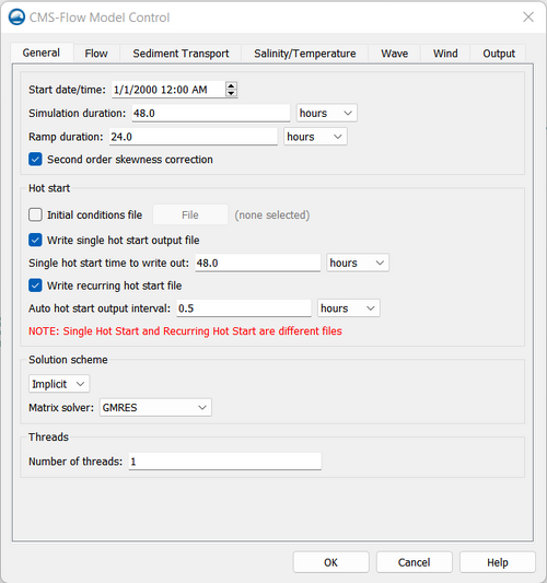
All of the CMS-Flow model parameters, settings, and output options are controlled from the CMS-Flow Model Control window (Figure 1). The window has several tabs including the Flow tab in which most of the general settings are set for CMS-Flow. To open the CMS-Flow Model Control window, click on CMS-Flow | Model Control. The first tab will be the Flow tab. There are several sections within the tab including Time Control and Hot Start options.
General

Time Control
Below are some of the CMS cards related to the Time Control of the Flow tab. Table 1 provides a brief description of the CMS cards used for time control. Figure 2 shows the time parameters in CMS-Flow.
| Card | Arguments | Default | Range | Description |
|---|---|---|---|---|
| STARTING_JDATE | REAL | none | none | Julian data in YYDDD with YY being last two digits of the year, and DDD the Julian day of the year. |
| STARTING_JDATE_HOUR | REAL | none | none | Julian hour . |
| HYDRO_TIME_STEP | REAL | Calculated based on solution scheme and courant number | none | Sets to the time step for hydrodynamics in seconds. |
| DURATION_RUN | REAL | 48.0 | >RAMP>0 | Sets the duration of the model simulation in hours. |
| DURATION_RAMP | REAL | 1.0 | Sets the length of the ramp period in which the model forcing is slowly ramped from zero. |
Hot Start
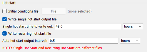
The term Hot start (Figure 3) refers to starting a simulation with an initial condition other zero (cold start). Hot starts are used for specifying initial conditions or restarting simulations at intermediate times. The hot start controls are set in the Flow tab of the CMS-Flow Model Control window.
Hot Start File
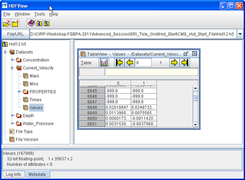
The CMS hot start feature CMS lets the user restart simulations that have been stopped due to electric outages, hardware malfunctions, or model crashes. In the case of a model crash the user, may restart the model using larger solver iterations and/or time steps to stabilize the simulation. The user has the option to specify a hot start output time or an interval for outputting a recurring hot start file. Every time the hot start file is written, it overwrites the previous information. The CMS Hot Start file saves information on the water elevation (pressure), and current velocities. If the sediment transport is active, then the water depth and sediment concentrations are also saved for each size class. Only the very last record of information is preserved (no starting from earlier intervals).
The CMS hot start files are written as binary XMDF files by default. Depending on the type of hot start (single file or recurring), the names are as follows are saved in the directory of the CMS-Flow files:
- SingleHotStart.h5
- AutoHotStart.h5
After saving a CMS Hot Start file, it is a good idea to rename the file with a different name before using it as an initial conditions file. This way, the file will not be overwritten in future simulations.
Table 1. Hot Start CMS-Flow Cards
| Card | Arguments | Default | Range | Description |
|---|---|---|---|---|
| HOT_START_TIME | REAL | none | none | Single time after start at which to output a single hot start file. |
| AUTO_HOT_START_INTERVAL | REAL | none | none | Sets the recurring hot start output interval . |
Initial conditions file
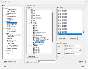
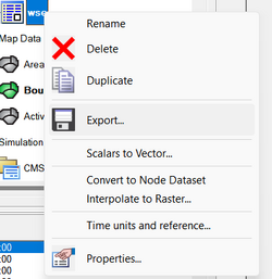
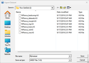
There are several situations where it is convenient to specify a user defined initial condition (hot start) file. For example, if the user forgets to setup the model output a hot start file or when running idealized cases with known initial conditions. A hot start file can easily be created and exported by the user from the SMS interface. The model requires at water levels, current velocities, concentrations, and water depths. Any datasets that are missing from the initial file are assigned a default value which depends on the dataset. If the water level or current velocities are not specified, they are set to zero. If the depth is not specified, then it is set to the input grid depth. If the sediment concentrations are not specified, then they are set to the equilibrium concentrations. It is important to note that the names and paths of the initial condition datasets are important.
| Variable | Path and name |
|---|---|
| Water surface elevation | Datasets\Water_Elevation |
| current velocity | Datasets\Current_Velocity |
| Sediment concentrations | Datasets\Concentration |
| Salinity concentrations | Datasets\Salinity |
Steps for creating a user defined hot start or initial condition file
- 1. Import CMS-Flow grid and solution file.
- 2. Sample a time step of the solution datasets for use in the initial condition
- Click on Data | Data Calculator (Figure 5)
- Under the Tools section, select Sample time steps.
- Under the Datasets section, click on the variable desired to be save (water surface elevation, current velocity, sediment concentrations or salinity concentrations)
- 3. Export the initial condition datasets to an XMDF file (Figure 6)
- Write Hot Start output file [On/Off]
- Automatic recurring Hot Start file [On/Off]
Solution Scheme

This refers to the temporal discretization of the hydrodynamic, sediment and salinity transport equations. There are two options in CMS: implicit and explicit. CMS-Flow has both implicit and explicit solution schemes.
Implicit
CMS-Flow implicit uses a generic Cartesian grid which can be regular, nouniform, or locally refined by splitting cells into two or four (only splitting into four supported by the interface at moment). Only three requirements are im-posed on the input grid: CMS-Flow Computational Grid
- 1. Cells must have a rectangular shape. Irregularly shaped cells are not allowed.
- 2. Cells may have a total of four to six neighboring cells (faces).
- 3. Only two cells are allowed in the same neighboring direction (i.e. North, South, East, West).
Explicit
The explicit solver is designed for dynamic problems with extensive wetting and drying which require small computational time steps, while the implicit solver is intended for simulating tidal and wave-induced circulation at tidal inlets, navigation channels, and adjacent beaches. A detailed description of the theoretical and numerical formulation of the explicit solver can be found in Buttolph et al. (2006) and is not repeated here. The sections below refer to the implicit solver.
The influence of the sub-grid scale turbulence can be particularly relevant in these situations. The implicit hydrodynamic model is capable of handling subcritical, transcritical and supercritical flow regimes but may require a very small time for transcritical and super-critical flows making the computation making the model inefficient.
For flows with a high Froude number, it is recommended to use the explicit flow model. Flow through structures is handled using empirical equations.
Matrix Solver
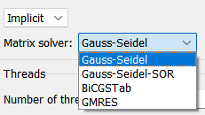
Matrix solver (Figure 8):
Threads

- Number of threads (Figure 7)
The CMS-Flow is parallelized for PC’s with multi-core processors using OpenMP. The number of threads used for parallel processing. The parallelization works by splitting the computational work into “threads” among several cores. Some cores are hyper-threaded, meaning a single core may support two threads. The number of threads is specified in the CMS-Flow Model Control Window. The number of threads must be equal or greater to 1 and cannot be larger than the number of threads available on the machine. If a number is specified which is larger than the maximum number available on the machine, then the code will default to the maximum number available.
For more detail, see Multi Processor Capability
Reference: CMS User Guide 013
Flow
In the Flow tab inside the CMS Flow, users can specify parameters and variables that will be used in the simulation. For example, in this section the Coriolis effect is assigned, friction coefficients and turbulence models are chosen.
Parameters

- Hydrodynamic Time Step
- Wetting and drying*
In the numerical simulation (Figure 10) of the surface water flows with sloped beaches, sand bars and islands, the water edges change with time, with part of the nodes being possibly wet or dry. In the present model, a threshold flow depth (a small value such as 0.02 m in field cases) is used to judge drying and wetting. If the flow depth on a node is larger than the threshold value, this node is considered to be wet, and if the flow depth is lower than the threshold value, this node is dry. Because a fully implicit solver is used in the present model, all the wet and dry nodes participate in the solution. Dry nodes are assigned a zero velocity. On the water edges between the dry and wet nodes, the wall-function approach is applied.
- Wave Fluxes and Roller Fluxes
User can check the options for wave and roller fluxes if wave outputs are desired.
- Average latitude for Coriolis
Specifies the average latitude for the grid which is used for the Coriolis parameter. If specified and average latitude is calculated for the grid and used to estimate the Coriolis parameter. By default, the cell latitudes are stored in the XMDF Model Parameters File. For additional details on this file see XMDF CMS-Flow Model Parameters File (*_mp.h5). For more details, see [1] Reference: Geospatial Information More information and tests: [2][3]
Bottom and wall friction
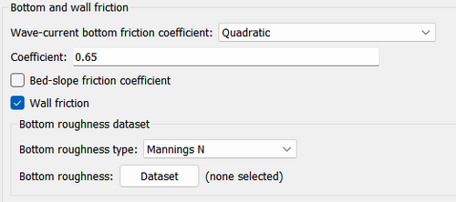
In this section, users may specify wave current bottom friction and roughness dataset (Figure 11).
Bottom roughness dataset
The bottom roughness type (Mannings N, Bottom Friction Coefficient, or Roughness Height) may be specified using a grid dataset referred to as the Bottom Friction Dataset. The dataset contains spatially variable or constant values and is the most general way of specifying the bed roughness. A description of the CMS-Flow cards related to the Bottom Friction Dataset are shown in the table below.
The bottom roughness is specified in the Bottom Friction Dataset section of within the Input tab of the CMS-Flow Model Control window. The Bottom roughness is specified at every computational (ocean) cell and is required for each model simulation. In SMS 11.1, the bottom friction dataset is specified in the Flow tab of the CMS-Flow Model Control window (see Figure 2 23). As in SMS 11.0, the bottom roughness can be specified as a roughness height, bottom friction coefficient, or in Manning's n coefficient. [4]
For the wave-current bottom frictions coefficients, five options are available (Figure 12):

- Quadratic
- Soulsby (1995) Data 2
- Soulsby (1995)Data 13
- Fredsoe (1984)
- Huyn-Thanh and Temperville (1991)
For more details, see Bottom Friction See How to create a bottom friction dataset
Turbulence parameters

Users can choose different Turbulence Model: Subgrid, Falconer, Parabolic or Mixing length (Figure 13). IT is not recommended to edit the default turbulence parameters. For more details, see Subgrid Model [5]
Edit turbulance parameters
Edits in this section are not recommended.
Sediment Transport
Timing
Users can determine from which CMS-Flow will start calculating the morphology change (Figure 14). The default value is 0 hours

Formulation

The formulation option available in CMS Flow is the Nonequilibrium total load (Figure 15. For more information, see:
Transport formula
There are five transport formulas to calculate the morphology change (Figure 16).

- Lund-CIRP
- Van Rijn
- Soulsby-van Rijn
- Watanabe
- C2SHORE
For a detail explanation, see:
Properties

Default values for the sediment density and porosity (Figure 17) are given. For more information, see:
Bed Composition
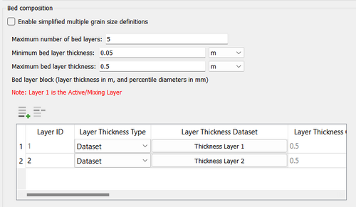
In these sections (Figure 18), users can choose to run the model with the simplified grain size definitions.
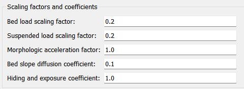
Scaling factors and coefficients
Adaptation

The adaptation coefficient (Figure 20) is an important parameter to consider in setting up the CMS sediment transport model. The sensitivity of results to the adaptation coefficient depends on the spatial and temporal scales of the problem. For example, if a high-resolution grid is used to model short-term dynamics of a nearshore disposal site or a small inlet, then the adaptation coefficient is likely to be important. However, if a relatively coarse grid is used to study sediment pathways in a large estuary entrance, then the adaptation coefficient will not be important, [7]
Transport grain sizes classes
Avalanching

Avalanching is the process of sediment sliding when the critical angle of repose is reached (Figure 21). In CMS, avalanching is simulated using a mass conservative relaxation method which limits the bed slope to the critical angle of repose. For most coastal applications, the critical angle of repose is never reached, so it is not needed. The CMS-Flow cards used for specifying avalanching, and its options, are described in table below.[1] Avalanching is invoked if the bottom slope between two cellsexceeds a specified critical slope. The avalanching algorithm applies an iterative approach to move material down slope until the critical slope is no longerexceeded, while conserving sediment volume. [2]
Hard Bottom

The sediment transport and bed change equations assume a loose bottom in which the bed material is available for entrainment. However, hard bottoms may be encountered in practical engineering applications where bed materials are non-erodible, such as bare rocks, carbonate reefs, and concrete coastal structures. Hard-bottom cells in CMS are handled by modifying the equilibrium concentration as in both the sedment transport and bed change equations. The bed-slope term in the bed change equation is also modified so that only deposition (no erosion) may occur at hard-bottom cells. [6]
Although the hard bottom dataset can be edited (when its the active dataset) by selecting a cell (or group of cells) and changing the scalar (S) value in the Edit Window, an user-friendly window exists which provides specification options. With the Select Grid Cell tool active, make a selection, right click to bring up the tool menu and choose the Specify Hard Bottom... option. This will open the CMS-Flow Hard Bottom Specification window. [7]
The following options are provided in the Hard Bottom Specification window:
- Use bathymetric cell depth - Sets the cell hard bottom depth to be the cell geometry value thereby creating an exposed non-erodible condition. If multiple cells were selected, then each cell will use its respective bathymetric depth.
- Specified distance below bathymetric cell depth - Sets the cell hard bottom depth to be the cell geometry value plus the specified distance thereby creating a sediment-covered non-erodible condition. The distance is limited to positive values to ensure the hard bottom depth is greater than the geometry value. The cell can provide sediment for transportation, however, the amount of erosion is limited. If multiple cells were selected, then each cell will use its respective bathymetric depth.
- Specified depth - Sets the cell hard bottom depth to the specified depth thereby creating a sediment-covered non-erodible condition similar to specified distance. The depth is limited to greater than the geometry value. If multiple cells were selected, then the depth is limited to greater than the largest geometry value and all cells will have the same value.
- Unspecified - Resets to an inactive hard bottom condition. The cell hard bottom depth is set to the CMS-Flow null value. If multiple cells were selected, then all cells will be reset.
If no cells are selected when opening the Hard Bottom Specification window, then all computational (ocean) cells will be used. If a selection of only non-computational cells, then specification cannot occur. If a selection contains computational and non-computational cells, then the specification will only apply to the computational cells.
If multiple computational cells with differing specifications are selected, the window will not display a selected specification type and the OK button will be disabled. This is to protect the previous specifications from being overwritten by mistake. The OK button will be enabled when an option is selected. The minimum hard bottom depth of the multiple computational cells selected will be displayed in the Depth edit field and the minimum hard bottom depth minus the maximum geometry depth of the multiple computational cells selected will be displayed in the Distance edit field.
Salinity/Temperature
The general parameters are the water density and temperature. The CMS-Flow cards for the general parameters are described in the table below.
Water properties

- Wave information
- Extrapolation distances
Salinity
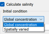
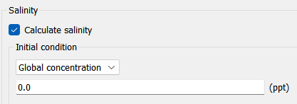
The characteristics of salinity are important in the coastal environment because salinity can impact marine plants and animals and influence the dynamic behavior of cohesive sediments. Because modifications of coastal inlets, such as channel deepening and widening and rehabilitation or extension of coastal structures, may alter the salinity distribution within estuaries or bays, it is often useful and convenient to simulate the salinity within the scope of an engineering project to determine if a more detailed water quality modeling study is necessary. It is important to emphasize that the CMS is not intended to be used as a water quality model. The CMS solves the depth-averaged (2DH) salinity transport equation and should be used only for cases where the water column is well mixed. If there is flow stratification, a 3D model should be utilized. It is also noted that the salinity is not used to update the water density which is assumed to be constant. Thus any horizontal water density gradients due to varying salinity on the hydrodynamics are assumed to be negligible.2
Temperature
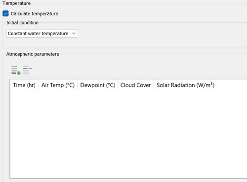
The properties of sea water are a function of temperature, salinity (i.e. dissolved minerals) and pressure (Figure 23). The water density and dynamic viscosity (kinematic viscosity times the water density) are shown in the following two figures as a function of water temperature and salinity. 10
Table 1. CMS-Flow cards related to the general parameters
| Card | Arguments | Default | Description |
|---|---|---|---|
| WATER_DENSITY | REAL | 1025 | Water density in kg/m^3. |
| WATER_TEMPERATURE | REAL | 15 | Water temperature in degrees Celcius. |
Wave
Wave information
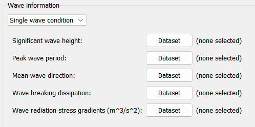
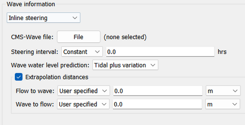
In this module, users may assign wave values or insert the simulation files from CMS Wave (.sim).
Extrapolation distances
Wind
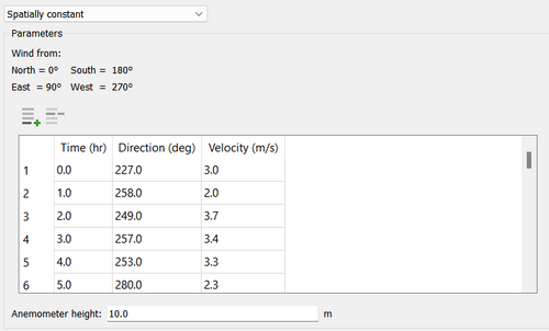
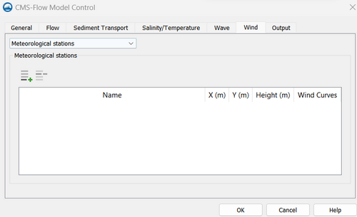
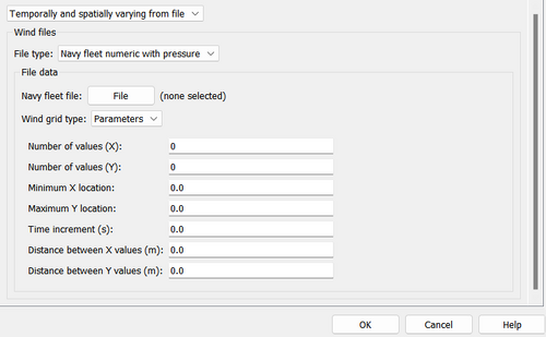
Users can insert Wind forcing into the model with three different methods:
Spatially constant
Meteorological stations
Temporally and spatially varying from file
For more details, see CMS Flow Wind Forcing
Output
Output time lists
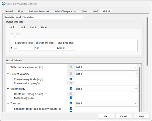
Users may specify different time intervals for the multiple outputs of CMS Flow. Different lists with different timeframes can be created and be assigned to specific outputs. For more information, see: CMS Flow Output
