Utilities

Time Series Analysis

filter1d.m

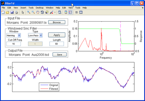
Filter1D: Time Series Analysis Tool

• The Matlab utility provides users of the SMS, a one-stop package for preparing model input time series and allows users to interpolate, resample, filter, and transform any type of model forcing and supports SMS compatible file formats for ease of data transfer.
• The main feature of the software is the ability to apply high-pass, low-pass, band-pass, and band-stop filters to time series.
• Filter1D uses a windowed sinc filter which is a non-recursive finite impulse response filter.
• Wiki Manual Filter1d
• PDF User Guide filter1d_user-guide.pdf
• Download Matlab script filter1d.m
• Download Matlab executable filter1d.exe
• Link to download Matlab Compiler Runtime library: http://www.mathworks.com/products/compiler/mcr/
• Download sample time series data file Blind_Pass.tsd

TAP Interface

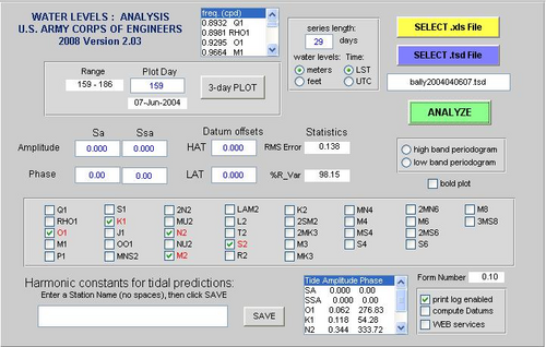
TAP: Tidal Analysis and Prediction software

• TAPtides is the ideal package to explore and develop preliminary or finalized tidal predictions from serial records spanning several weeks to several months.
• Designed to be easy to use, its Graphical User Interface permits quick separation of a time series of water level measurements into its tidal and non-tidal components using a selective least squares harmonic reduction employing up to 35 tidal constituents.
• After saving the tidal constants for the constituents selected during analysis, the user can generate predictions of the astronomical tide, the water level that varies at known tidal frequencies attributable to gravitational interactions between the earth, moon, and sun.

• Wiki Manual for TAPtides TAPtides
• Wiki Manual for TAPcurrents TAPcurrents
• Download software TAP.rar

Matlab scripts

Read CMS-Flow Grid File (*_grid.h5)

cms_read_grid.m Reads a CMS nonuniform Cartesian grid

• Description:

Reads a CMS grid file and creates a structure variable containing the grid variables

• Usage:

grd = cms_read_grid(filename);

• Input:

filename - Input file name including full path (e.g. 'Flow_grd.h5')

• Output:

grd - structure variable containing the following variables

nx - Grid size in x direction [-]

ny - Grid size in y direction [-]

x0 - Grid origin in x direction [m]

y0 - Grid origin in y direction [m]

angle - Grid angle [deg]

x(1:nx) - Cell-center coordinates in x direction [m]

y(1:ny) - Cell-center coordinates in y direction [m]

depth(1:ny,1:nx) - Cell-centered depth [m]

active(1:ny,1:nx) - Cell activity (1-active and 0-inactive) [logical]

Plus other optional datasets such as mannings, d50, etc.

• Author: Alex Sanchez, USACE-ERDC-CHL

• Download Matlab script - cms_read_grid.m

Read CMS-Flow Tel File (*.tel)

• Description:

Reads a CMS telescoping grid file and output all variables to a structure array.

• Usage:

out = cms_read_tel(telfile);

• Input:

telfile - Telescoping grid file including path (*.tel)

• Output:

tel - Structure including the following fields

ncells - Number of cells

x0 - Grid origin in x-direction [m]

y0 - Grid origin in y-direction [m]

angle - Grid angle [deg]

id - Cell ID number

x - Grid cell-centered coordinate in x-direction [m]

y - Grid cell-centered coordinate in y-direction [m]

dx - Grid cell resolution in x-direction [m]

dy - Grid cell resolution in y-direction [m]

iloc - Cell connectivity

depth - Cell-centered depths (-999 = inactive cell) [m]

• Author: Alex Sanchez, USACE

• Download Matlab script - cms_read_tel.m

Read CMS-Flow solution files

• Description:

Reads a CMS solution file and creates a structure variable containing the solution datasets values and times

• Input:

filename - input file name including full path

grd - Grid structure containing the following fields

nx - Grid size in x direction

ny - Grid size in y direction

varargin - dataset names

• Output:

sol - structure variable containing dataset values and times

varargout - variable length datasets corresponding to varargin

• Usage:

filename = 'test_sol.h5';

sol = cms_read_sol(filename,grd);

wse = cms_read_sol(filename,grd,'Water_Elevation');

[wse,uv] = cms_read_sol(filename,'Water_Elevation','Current_Velocity');

sol = cms_read_sol(filename,'grid',grd,'datasetnames',dnames,...

'points',pts,'cells',ids,'polygon',poly,'steps',nstep,'times',t)

• Author: Alex Sanchez, USACE-ERDC-CHL

• Download Matlab script - cms_read_sol.m
• Download sample solution file test_sol.h5

Read SMS Time Series Data File

• Description: Reads the Surface-water Modeling System time-series data (*.tsd) file.
• Usage:

[t,dat,name,units] = sms_read_tsd('data.tsd');

• Download Matlab script - sms_read_tsd.m.

Read a CMS Save Point File

• Description:

Reads a CMS Save Point file

• Usage:

sp = cms_read_sp(filename);

• Input:

filename - CMS Save Point file name

• Output:

sp - Structure with the following fields

variable - Name of output variable

reference_time_str - Reference time string in the following format 'yyyy-mm-dd HH:MM:SS'

reference_time - Reference time

label - Save point label

creation_date - Creation date

horizontal_projection - Horizontal projection

vertical_datum - Vertical datum

time_units - Time units

output_units - Units of output variable

cms_version - CMS version number

number_points - Number of points in time series

names - Names of output points

xy - Coordinates of output points

time - Output times

scalar - Output scalar

vector - Output vector

• Author: Alex Sanchez, USACE-CHL

• Download Matlab script - cms_read_sp.m.

Write SMS Time Series Data File

• Description: Writes a Surface-water Modeling System time-series data (*.tsd) file.
• Usage:

sms_write_tsd(filenamet,dat,curvename,curvetype);

• Download Matlab script - sms_write_tsd.m.

Read SMS XY Series File

• Description: Reads the Surface-water Modeling System xy series (*.xys) file.
• Usage:

[x,y,name] = sms_read_xys('data.xys');

• Download Matlab script - sms_read_xys.m.

Write SMS XY Series File

• Description: Writes a Surface-water Modeling System xy series (*.xys) file.
• Usage:

sms_write_xys(file,x,y,name)

• Download Matlab script - sms_write_xys.m.

Bin scatter data

Example of xyzbin.m application to multibeam data with 5-m bins.

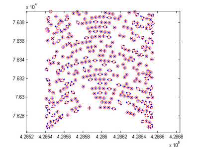
• Description: Averages the x, y, and z values of points within the same bin. The grid used to define the bins may be user specified are calculated based on the extent of the scatter points. The routine is useful for thinning/smoothing large scatter sets such as multibeam or LIDAR data. The binning method is less accurate then the search radius method, but is much faster.
• Usage:

[x,y,z] = xyzbin(...);

[x,y,z] = xyzbin('infile',infile,'outfile',outfile,'dx',dx);

[x,y,z] = xyzbin('x',xin,'y',yin,'z',zin,'dx',dx);

[x,y,z] = xyzbin('x',xin,'y',yin,'z',zin,'dx',dx,'dy',dy);

[x,y,z] = xyzbin('infile',infile,'dx',dx,'x0',x0,'y0',y0,'theta',theta);

• Download Matlab script - xyzbin.m.

Interpolation of CMS-Wave Spectra

• Description: Interpolates the energy spectra in the CMS-Wave *.eng file to a specified output interval which may be specified in intervals or time units (hours). For example, an output interval of 0.5 index units, interpolates the spectra at half intervals. This subroutine is useful for filling small gaps in CMS spectra.
• Usage:

interp_eng('Wave.eng','New.eng',1,0.5) %interpolates to every half interval

interp_eng('Wave.eng','New.eng',1,2) %resamples every two spectra

interp_eng('Wave.eng','New.eng',2,1) %hrs

• Input:

engin = Input eng file

engout = Output eng file

mode = 1 - Index, 2 - Time

dtout = Output steering interval in hours for mode=2 or index for mode 1 (can be less than 1)

• Download Matlab script - interp_eng.m.

Principle Component Analysis

Example of a principle component analysis.

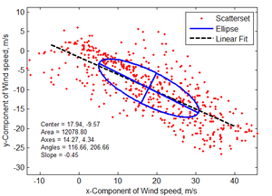
• Description: Calculates the principle axes of vector time series data. This subroutine is useful for determining the main direction of fluid flow and extracting the velocity component along the major axis. The principle axes are determined by solving the eigenvalue problem for two-dimensional scatter data.
• Usage:

s = pca2d(u,v)

• Output:

s = Structure with the following fields:

center = Ellipse center (centroid)

area = Ellipse area

axes = Ellipse axes

eigen_values = Eigen values

eigen_vectors = Eigen vectors

total_variance = Total variance

percentage_variance = Percentage variance for each axes

angles = Angles for each axes in degrees

eccentricity = Ellipse eccentricity

slope = Slope of the linear fit which goes through the origin

• Note: An alternative simple way of determining the principle axes of vector time series is

$\phi _{p}={\frac {1}{2}}\arctan ^{-1}{\biggl (}{\frac {2{\big \langle }u'v'{\big \rangle }}{{\big \langle }u'^{2}{\big \rangle }-{\big \langle }v'^{2}{\big \rangle }}}{\biggr )}+\pi /2$

(1)

where $u'=u-{\bar {u}}$ and $v'=v-{\bar {v}}$.

• Download Matlab script - pca2d.m:.

Data Density Scatter Plot

Example of a data density plot.

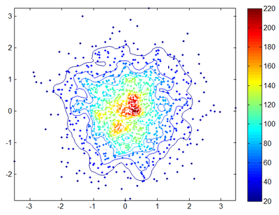
• Description: datadensity Computes and plots the data density (points/area) of scattered points
• Usage:

dd = datadensity(x,y,method,radius)

• Input:

(x,y) - coordinates of points

method - either 'squares','circles', or 'voronoi'

default = 'voronoi'

radius - Equal to the circle radius or half the square width

• Download Matlab script - datadensity.m:.

Spectral Analysis

Example of Power Spectrum for an idealized water level time series with white noise and a large gap.

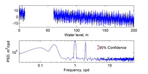
• Description: Calculates the spectrum for a scalar time series using Welch's method. The confidence intervals are calculated with the inverse of chi-square distribution. Also includes a filtering option using the butterworth filter to see the effect of the filter on the spectrum.
• Usage:

q = specwelch(x,dt,w,Nsg,pnv,Wn,ftype,n);

[psdf,f] = specwelch(x,dt,w,Nsg,pnv,Wn,ftype,n);

[psdf,conf,f] = specwelch(x,dt,w,Nsg,pnv,Wn,ftype,n);

• Input:

x - Time series, [vector]

dt - Sampling Rate, [scalar]

win - Window, one of: 'hanning', 'hamming', 'boxcar'

Nsg - Number of Segments (>=1)

pnv - Percentage Noverlap of Segments (0-100)

Nb - Band Averaging, number of bands to average

P - Probability for confidence intervals, (e.g. 0.95)

Wn - Cut-Off frequencies, used for filtering

ftype - Type of filter, 'high', 'low' or 'stop'

n - Number of coefficients to use in the Butterworth filter

• Output:

q - structure with the following fields:

xp - detrended x

f - Frequencies

T - Periods

m - Magnitude

a - Amplitude

s - Power spectrum, Sxx(win), [Power]

psdw - Power Spectrum Density, Pxx(win), [Power/rad/sample]

psdf - Power Spectrum Density, Pxx(f), [Power/sample-freq]

psdT - Power Spectrum Density, Pxx(T), [Power*time-unit]

conf - Upper and Lower Confidence Interval multiplication factors using chi-squared approach

• Download Matlab script - specwelch.m.

Vector Plot

Example comparisons between feather.m, quiver.m, and vecplot.m

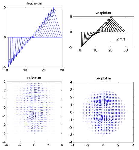
• Description: Plots directionally correct vectors. Both of Matlab subroutines feather.m and quiver.m do not preserve the correct vector angles.
• Usage:

h = vecplot(x,y,u,v,'PropertyName',PropertyValue,...)

h = vecplot(u,v,'PropertyName',PropertyValue,...)

• Input:

x,y = Position Coordinates

u,v = Vector Componentes

• Optional Properties

'DataAspectRatio' = Scaling factor between x and y axes. This is set as the second element of the property 'DataAspectRatio'

'LengthScale' = Length scaling factor for the barbs or arrows

'LineSpec' = Line specification string syntax (default '-k^') (e.g. '^k' - plots black arrows, 'k' - plots black sticks)

'Linewidth' = Linewidth

'Marker' = '^' for triangle arrows, 'v' for angled arrows,

and for stick plots (default stick)

'MarkerFaceColor' = Arrow fill color (default none)

'MarkerEdgeColor' = Arrow edge color (default line color)

'MarkerSize' = Marker size

'LegendLength' = Sets the length of the legend vector

'LegendUnits' = Sets the units for the legend vector

'legendPosition' = Sets the legend position (normalized units 0-1)

• Output:

h = handles for plot objects

• Download Matlab script - vecplot.m.

Example using vecplot to plot wave conditions.

Tidal Harmonic Analysis

Example tidal harmonic analysis results for Crescent City, CA

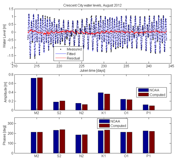
• Description: Simple program which performs a tidal harmonic anlaysis of scalar (e.g. water level) or vector (current velocity) time series. The script is only applicable for relatively short time series of a few months.
• Usage:

out = tha(in);

• Input:

in - Structure array with the following fields

x - real or complex vector [arbitrary units]

t - time in hrs from zero [hours startin from zero]

start_time - starting time as [yyyy,mm,dd,HH,MM,SS]

constituents - optional input constituent names

rayleigh - optional rayleigh criteria (<=1)

secular - optional secular correction. Either 'linear' or 'none'. If set to 'linear', the slope is included as a correction to the time series.

• Output:

out - Structure array with different fields depending on whether the input time series in real or complex.

amplitudes - Tidal constituent amplitudes (real time series)

constituents - Tidal constituent names

equilibrium_arguments - Equilibrium arguments (v+u) for each constituent and starting time

frequencies - Tidal constituent frequencies

frequency_units - 'cycles/hour'

nodal_factors - Nodal factors for each constituent and year.

phases - Tidal constituent phases

phase_units = 'degrees'

percent_variance_explained - Percent variance explained of the measured time series by the fitted time series.

residuals - difference between measured and fit time series

slope - fitted slope(s)

speeds - Tidal constituent speeds in degrees/hour

speed_units = 'degrees/hour'

time - Julien time in hours from start of year

time_units = 'hours'

(variables bewlow are only for complex time series only)

major_amplitude - Semi-major axis amplitude

minor_amplitude - Semi-minor axis amplitude

positive_amplitude - Positive axis amplitude (a+)

negative_amplitude - Negative axis amplitude (a-)

positive_phase - Positive axis phase (phase+) [deg]

negitive_phase - Negative axis phase (phase-) [deg]

ellipse_inclination - Ellipse orientation or inclination [deg]

eccentricity

• Version: 3.0
• Date: November 5, 2012
• Author: Alex Sanchez, USACE-CHL
• Download Matlab function tha.m.
• Download Matlab test script tha_test.m.
• Download tidal data file with nodal factors and equilibrium arguments tide_data_v1.mat.
• Download sample time series file for Crescent City, CA TimeSeries_9419750.txt.
• Download sample constituent file for Crescent City, CA Constituents_9419750.txt.

Extract Time Series from NOAA World Blended Sea Winds

• Description: Extracts a time series of wind speed and direction for use in CMS from the 6 hrly global blended sea wind database (http://www.ncdc.noaa.gov/oa/rsad/air-sea/seawinds.html) which has a 0.25º resolution. Outputs *.xys files which can easily be imported into SMS.
• Download Matlab script - blended_winds_extract_time_series.m

Blended Surface Sea Winds for a section of the North-West US coast.

Extracted sea winds

Extracted sea winds

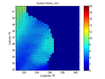
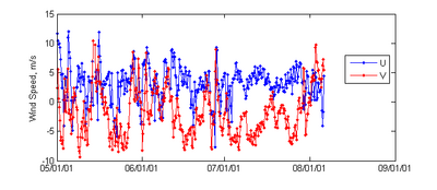
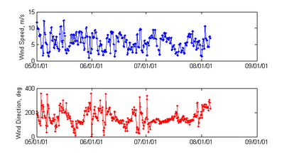
Image Digitization Tool

Example digitization of an earthquake rupture zone.

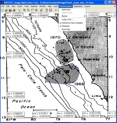
• Description: digitize is a user interfase that allows to import image files (.bmp, etc) into MatLab to digitize data from. Previous sessions can also be loaded. It is useful for digitizing plots%and making world files for images. The utility can be used for digitizing time series plots, geographic features such as coastlines, or elevation contours.
• Instructions:

• Load image

1. To start a new session, click on the "Load" menu and select "Image File".
2. To load a saved session, click on the "Load" menu and select "Session".

• Reference the image

1. Click on the "Transformation" menu and select "Add Points".
2. Left-click on the points reference points and Right-click when finished.
3. Right-click on any reference point and select "Reference" to enter the points "true" coordinate.
4. When the coordinated for all the reference points have been entered the "Reference Data Complete" item under the "Transformation" menu will be checked.
5. To delete Transformation points, right-click on a point and select "Delete".

• Digitize Points

1. Click on the "Digitization" menu and select "Add Points". The digitized points may be entered at any time, but their transformed coordinated are not calculated until the reference data is complete.
2. To see a digitized point's transformed coordinate, right-click on a point and select "Coordinates".

• Export the Digitized Points

1. Click on "Export" and select one of the output options including variables to the workspace and an ASCII file.

• Download Matlab script - digitize.m.

Create Spectra Generation Import file with WIS datafiles

• Description: This function creates the .txt file used in the spectra generator of CMS Wave. It prompts the user to select all the desired WIS output files, specify the depth of the station, and whether or not to average the data series. The data and user inputs are manipulated into the format used by CMS Wave file import for spectra generation. Currently the output file is saved in the active directory of matlab.
• Usage: Type mfile name in Matlab command window

CMS_WIS_to_txt_for_spectragen

• Download Matlab script - CMS_WIS_to_txt_for_spectragen.m.

Read an SMS Super ASCII data file (*.dat)

• Description: This function reads an SMS Super ASCII data file (*.dat). These files are part of the SMS Super ASCII format and is an output option for global solution datasets in CMS. The SMS Super ASCII format also includes a coordinates file (*.xy) and a super file (*.sup) which contains the names of the coordinate file and dataset files.
• Usage:

[t,x] = readsuperdat(filename);

• Download Matlab script - readsuperdat.m.

Read an SMS xy file (*.xy)

• Description: This function reads an SMS xy file (*.xy). These files are used in the SMS Super ASCII in conjuction with the by CMS as an ASCII output option for global solution datasets. The SMS Super ASCII format also includes dataset files (*.dat) and a super file (*.sup) which contains the names of the coordinate file and dataset files.
• Usage:

[t,x] = read_xy(filename);

• Download Matlab script - read_xy.m.

Wave Number Calculation

• Description: Simple program which solves the wave dispersion relation sig^2 = g*k*tanh(k*h).
• Usage:

wk = wavenumber(g,wa,wd,h,u,v,tol)

[wk,err] = wavenumber(g,wa,wd,h,u,v)

• Download Matlab script - wavenumber.m.

Read Sediment Flux

• Description: Reads in data from CMS sediment flux output file, skipping header lines.
• Usage:

data = read_sed_flux(filename)

• Input:

no arguments - use ui to select file manually

one argument (<filename>) - input file name (as a string). If path is not specified it will be assumed to be the present working directory.

• Output: data - a double in which each column represents a column from the file.
• Download Matlab script - read_sed_flux.m'

New CMS Tools menu (v5.2.5 and later)

This is a tool which works from the Command Line for CMS. Run '<cms executable> Tools' to get the menu. Note: depending on version number, certain options may not have been added yet. For all, get the latest version.

Print RT_JULIAN/REFTIME corresponding to actual date

This option will prompt the user for a date and will return an reference number.

For example, the date 2022-08-05 00:00:00:00 returns the value 983103.50

Print actual date corresponding to RT_JULIAN/REFTIME

This option will prompt the user for reference time and will return the actual date it corresponds to. This is useful for some ASCII Output from CMS that contains this value.

For example, the reference time 983103.50 returns the date 2022-08-05 00:00:00:00

Read WSE Dataset and output a Max WSE dataset for all times

• This prompts the user to enter the filename for a water surface elevation solution file which was output from a CMS simulation.
• It then reads all times for all cells in the file and then writes a new solution file that contains one record which is the Maximum value for each cell in the grid over the entire simulation run. Can be used to see the maximum surge from storms or other events.
• The resulting file has the same prefix as other solution files but ends with '_maxwse.h5'.

Take multiple solution datasets and merge into one file

Many times a user will have several different files containing one or more datasets and they wish to pick and choose certain datasets to combine into one new file. This may be for use with PTM or perhaps the Sediment Mapping feature of CMS.

• The tool asks how many solution datasets to merge into a new file.
• Using the number from the first step, the code asks for the filename containing the datasets that the user wishes to merge into the new file.
  • Once the name is entered, CMS reads the file and presents a list of datasets names for the user to choose from.
  • The user will then choose which of the numbered datasets they want from the list.
• The tool then asks the user for the name of the merged file. Warning - an existing file of that name will be overwritten.
• The tool then displays the progress as it processes each of the selected datasets and then writes out the new file containing all of the data from the selected files.

Extract data for one cell from multiple datasets to a text file

Testing in progress.

TextPad Syntax File for CMS-Flow Card File

Example cmcards file viewed in Textpad

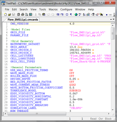
• Color codes the CMS-Flow card file (*.cmcards) so that it is easier to read and avoids misspelling of keywords.
• To setup the file:

1. Open Textpad and click on the menu Configure and go to Preferences.
2. Click on folder on the left hand side and note the path to the syntax files.
3. Copy-paste the .syn to the path noted in step 2.
4. Click on Configure | New Class Document.
5. Enter CMS-Flow as the document name and click next.
6. Enter *.cmcards in Class members and click next.
7. Enable the syntax highlighting and select the CMS-Flow_V4.syn file.
8. Click on Finish and your done!

• Version 4.0 and earlier: CMS-Flow_V4.syn.
• Version 4.1 and earlier: CMS-Flow_V4p1.syn.

Notepad++ Syntax File for CMS-Flow Card File

Example cmcards file viewed in Notepad++

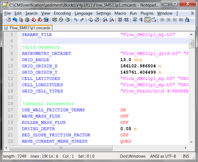
• Color codes the CMS-Flow card file (*.cmcards) so that it is easier to read and avoids misspelling of keywords.
• Version 4.1 and earlier: CMS-Flow_v4p1.xml.

UltraEdit Syntax File for CMS-Flow Card File

Example cmcards file viewed in UltraEdit

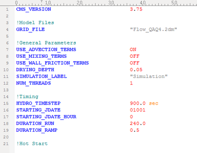
• Color codes the CMS-Flow card file (*.cmcards) so that it is easier to read and avoids misspelling of keywords.
• Version 4.1 and earlier: CMS-Flow_v4p1.uew.

HDFview

• HDFview is a free visualization tool for browsing and editing HDF4 and HDF5 files.
• To download or download a free copy visit:

https://www.hdfgroup.org/downloads/hdfview/

• Later HDFView binaries require C++ redistributables. If you install the viewer and still cannot access the files, try installing this:

https://support.microsoft.com/en-us/help/2977003/the-latest-supported-visual-c-downloads

Grain Size Distribution Analysis

• This Excel worksheet calculates statistics for many samples using several methods including Folk and Ward and the Method of Moments.
• Disclaimer: The analysis software GRADISTAT is developed by Kenneth Pyle Associates Ltd. This reference does not imply official or unofficial endorsement.
• Link: http://www.kpal.co.uk/gradistat.html

Wave Transformation

From Wave Characteristics to CMS-Wave spectral energy file.

Fortran executables for Windows

• Wave Watch III spectra
• WIS wave spectra
• CDIP Buoy wave spectra
• NDBC Buoy wave spectra

From 2D Spectra to CMS-Wave spectral energy file

Python source code

• WIS Stations

---

Documentation Portal