TAPcurrents
Tidal Analysis and Prediction of Currents: TAPcurrents
By John D. Boon and Alejandro Sanchez
Purpose
The wiki technical note herein describes the desktop computer program TAPcurrents for the tidal analysis and prediction of water currents in tidal waterways. Designed to be easy to use, its Graphical User Interface (GUI) permits quick separation of a time series of water current measurements into its tidal and non-tidal components using a selective least squares harmonic reduction employing up to 35 tidal constituents. After saving the tidal constants for the constituents selected during analysis, the user can generate predictions of the astronomical current, the water current that varies at known tidal frequencies attributable to gravitational interactions between the earth, moon, and sun.
Introduction
Many software packages are available today that allow current predictions to be made in tidal waters throughout the world. With few exceptions, these programs utilize tidal constants determined by governmental agencies and the casual user of this software is generally unaware of any of the details involved in the agency’s analysis, not least the breakdown of observed water current variation into its tidal and non-tidal parts. Separating water current histories into their tidal and non-tidal components is important for two reasons. It is easy to fault the astronomical prediction formula when predictions don’t agree with observations but, depending on the region, the astronomical current may in fact be quite small compared to wind-generated and other forms of locally induced current present in the same record. Very little information is available to users about the length of the current time series used to estimate tidal constants for predictions, or about how old the data are. Predictions for coastal waterways that have undergone significant hydrologic change (storms, dredging activity) are particularly susceptible to errors resulting from inadequate or outdated current measurements. Secondly, non-tidal currents are of interest in their own right, particularly in estuaries where gravitational circulation plays an important role in the transport of water-borne materials.
With the introduction of acoustic Doppler current monitoring devices, both governmental and non-governmental organizations have begun to acquire much more data than ever before. TAPcurrents is the ideal package with which to explore and develop preliminary to finalized current information from serial records spanning several weeks to several months. Although its operating features are intuitive and can be quickly grasped by users familiar with MS Windows® terminology, it is important to have a general understanding of the theory of tides and currents before using TAPcurrents. Comprehensive references such as Cartwright (2000) and Pugh (2004) are highly recommended for this purpose, as is Boon (2004) for a practical introduction.
Installation
To run TAPcurrents the MATLAB Component Runtime (MCR) program must first be installed using the MCRInstaller provided with the application package. When installing SMS select the option to install TAPtides and TAPcurrents. After unzipping the package in a working directory, right-click the TAPcurrents program icon to create a shortcut and place it on your desktop. Run the application by double-clicking on the icon: This will create a new folder with the required MCR programs.
TAPcurrents is programmed in the MATLAB® technical computing language, a product of The MathWorks, Inc. The present program is an executable version compatible with personal computers using the MS Windows operating system (Windows XP).
Data Formats
TAPcurrents accepts input data in either text format or Microsoft Excel format. The Excel format is recommended for users who collect original data from a variety of sources and require a platform that is convenient for manual data entry and editing (units conversion, date and time corrections, quality control parameters). The Excel workbook also provides multiple worksheets for inclusion of header information with location, sensor parameters, depth and other attributes of a self-describing data set. A text format is provided for a process-controlled data stream produced by the user’s own application.
Entering data with Excel
TAPcurrents input files may use an array of water current data entered on the first worksheet of a Microsoft Excel workbook with file extension .xls. Only files with this extension will appear when the ’SELECT .xls file’ button is pressed with the TAPcurrents Analysis page active (Fig. 1). Two Excel formats are available:
- 1. Polar format: current speed and direction
- Col. 1 - Date in Excel month-day-year format (mm/dd/yyyy)
- Col. 2 - Local Standard Time using Excel 24-hour format
- Col. 2 (Optional) Date&Time in Excel format: mm/dd/yy hh:mm
- Col. 3 - any non-numeric (e.g., 3-letter time zone label)
- Col. 4 - Current speed in meters per second or knots
- Col. 5 - Current direction in degrees 0-360 relative to true north
- 2. Vector format: east-west, north-south current speed components
- Col. 1 - Record number or profile number (numeric field)
- Col. 2 – Date & Time in Excel format: mm/dd/yy hh:mm
- Col. 3 – U (east-west) current component (meters/sec or knots)
- Col. 4 – V (north-south) current component (same per choice above)
- If serial date and time is used in column 2, a numeric value (e.g., Julian day) can be entered in column 1. A set of non-numeric column labels may be inserted as the first row of either array. Note that a 5th column is not allowed when using the vector format.
Entering data in Text Format
After pressing the button marked ’SELECT .tsd file’ while the TAPcurrents Analysis page is active, the user may use the browser to open a three-column ascii file containing either current speed (m/sec) and direction (degrees from true north) or U,V current components. TAPcurrents makes a determination based on the information contained in the second header string shown in double quotes below. Note that in lieu of time, the series utilizes a time offset in seconds after the starting date and time indicated in the third header string in double quotes. The two input formats for vector data are shown below
- TIME_SERIES
- "May 1, 2008" "Velocity - Mag. & Dir." 3 41 "05/01/2008 12:00:00"
- 0.0 1.0 -75.0
- 900.0 1.1 -70.0
- 1800.0 1.2 -65.0
- 2700.0 1.3 -60.0
- 3600.0 1.4 -55.0
- 4500.0 1.5 -50.0
- 5400.0 1.6 -45.0
- 6300.0 1.7 -40.0
- TIME_SERIES
- "Current Buoy 1" "Velocity - Components" 3 4376 "03/06/2003 14:45:00"
- 600.00 -0.494 0.03
- 1200.00 -0.525 0.052
- 1800.00 -0.546 0.06
- 2400.00 -0.542 0.051
- 3000.00 -0.576 0.058
- 3600.00 -0.6 0.073
- 4200.00 -0.601 0.069
- 4800.00 -0.597 0.058
Overview
The TAPcurrents menu has two options: Tidal Analysis and Tidal Prediction. The last two buttons launch programs to conduct water current analysis (TIDAL ANALYSIS) and generate tidal current predictions respectively (CHOOSING TIDAL CONSTITUENTS, TIDAL PREDICTION). The analysis portion of the software accepts several file types (see INPUT FILES). The files used in this CHETN are automatically downloaded during the installation process and are located within the TAPcurrents folder which is located in the SMS directory. The tidal prediction portion of the software requires tidal constituents (amplitudes and phases of individual tidal components) from the tidal analysis program.
Current Analysis
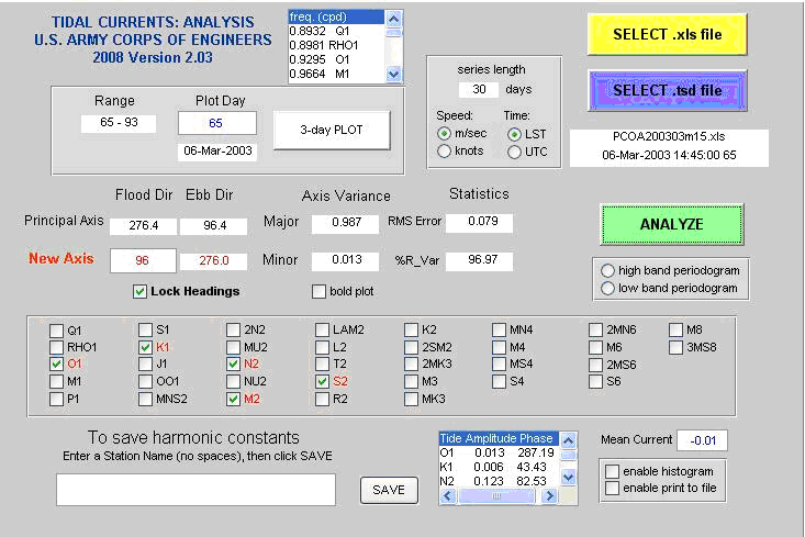
The method used by TAPtides to analyze a water current time series is commonly known as Harmonic Analysis, Method of Least Squares (HAMELS). It achieves a progressive reduction in variance (mean square deviation about the mean) by adding harmonic terms with specific astronomical frequencies to a general least squares model of the type used for multiple regression. It is not Fourier analysis, a procedure that employs only the Fourier frequencies. A brief description of HAMELS is given in Appendix B. For a complete description of the least squares harmonic analysis method employed here, the reader is referred to Boon (2004). Note that it is preferable to use the term water current analysis, rather than tide analysis, because the measured water currents in coastal waterways vary at both tidal and non-tidal frequencies. The objective of the analysis is to separate these components so that a tidal current prediction can be made with the component that is predictable – the water current that oscillates at tidal frequencies. Clicking the Current Analysis button within the SMS menu Tools|Harmonic Analysis starts the GUI page that performs water current analysis (see Fig. 1). It is recommended that the user click the Disclaimer menu at the top of the window and read the disclaimer message before proceeding. Click the Program Help menu immediately to the left of the Disclaimer button to view information about input files, file analysis, selection of tidal constituents and other topics. The analysis can then be undertaken with the following steps:
Settings and Selections
Check the appropriate units box (meters per second or knots) and press the file selection button to choose a data file in either the Excel (.xls) or text file format (.tsd). Using the browser, open one of the example files included with TAPcurrents and wait for the file to load and data graphics to appear. The main graphic that appears will contain a scatterplot of the U (east-west) and V (north-south) current components and the Principal Current Axis (PCA) of maximum variance. In multivariate analysis, the coordinate axis for the variable containing maximum variance is displayed as a blue line passing through the bivariate mean [Um,Vm]. Reciprocal headings for this axis may be viewed on the graphic as well as the flood and ebb direction boxes on the analysis page (Fig. 1). Normally the user will choose the heading corresponding to the flood direction and enter it in the edit box above the check box labeled ’Lock headings’, although another flood heading could be chosen as well (e.g., a channel axis). After entry, check ’Lock Headings’.
Lock Headings
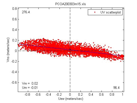
This step initiates a rotation of the U,V current axes about the U,V bivariate mean (black cross in Fig. 2) to align with the new heading. The rotation therein produces new orthogonal components, Up and Vp, in which Up readings along the major axis are positive in the flood direction and negative in the ebb direction. The ANALYZE button will turn green when ready to analyze Up as the variable with the largest part of the total variance (98.7% as shown in the Axis Variance text box in Fig. 1). Although the minor axis current Vp is ignored, this variable accounts for only 1.3% of the total variance in this case – not a large loss of information. Choosing Up, on the other hand, reduces the spatial dimensions of the plotting problem from two to one, thus allowing a visually informative current curve to be constructed in place of a vector diagram or a table of numbers. The ability to view the current curve in detail will be especially useful in the next stage of the analysis.
Analyze currents
The third step begins after pressing the large ANALYZE button on the right side of the page (Fig. 1). A new graph will quickly appear showing the results of a least squares harmonic analysis fitting the five main tidal constituents, O1, K1, N2, M2 and S2, to the Up current data. A listbox at the bottom of the page displays the tidal constants (amplitude and phase) computed for all five current constituents. The five symbols appear next to checked boxes inside a wide gray frame containing thirty more boxes left unchecked. The first five are always selected but the thirty others should be thought of as potential constituents that can be chosen for inclusion in the next round of analysis. After checking additional constituents, the ANALYZE button may be pressed again to perform another analysis.
Select constituents
Different regions have different tidal types which affects the number and importance of the tidal constituents represented in the current. The user must identify these constituents guided by the analytical tools provided in the Analysis GUI while recognizing that, for a relatively short series of observations (29 days to 58 days), there are limits to the number of tidal constituents that can be successfully resolved. In general, the difficulty caused by short series length arises in the resolution of certain constituents that are close to others in frequency (consult the list box at the top of the Analysis page for a list of available constituents and their frequency). The major solar semidiurnal constituent S2, for example, has a frequency of exactly 2 cycles per mean solar day (cpd); the semidiurnal constituents T2 (1.9973 cpd), R2 (2.0027 cpd) and K2 (2.0055 cpd) are all very close to this frequency and can be difficult to resolve in a short series.
The minimum series duration T necessary to fully resolve two tidal frequencies f1 and f2 is given by T =1/|f1-f2|, the synodic period. The synodic period for S2 and K2, for example, is 1/0.0055 or 181.8 days. Another important aspect to consider is the number of constituents chosen to model the tide. The user should start with the default constituents and carefully choose additional constituents on the basis of their ability to reduce residual variance without violating the synodic period rule. Likely candidates will be found using the high band periodogram to examine the total distribution of variance (energy) with frequency. The periodogram feature is further explained below.
3-day plot
After selecting constituents, the 3-day plot feature in the gray frame on the upper left side of the page can be very helpful. Like the main plot that appears after pressing the ANALYZE button, the 3-day plot uses Julian days to display time and select a time interval for plotting (the corresponding calendar date is also displayed for convenience). The 3-day plot of observed (red), predicted (blue) and residual (green) current gives a wave-by-wave view showing how well the tidal harmonic model fits the data. Obviously, the fit is very good if the residual is almost a flat line. However, when it is not and the blue curve starts showing double peaks while the red curve has only single peaks, this may be a further indication of the problem of trying too many tidal constituents with too little data.
Of course another reason to use the 3-day plot is to investigate errors; e.g., dropped data points, current speed shifts, or a shift to incorrect times. The least squares algorithm used in TAPcurrents is not affected by small data gaps, provided the time remains correct. This is one reason the data are entered in a multi-column spreadsheet – the user may check that every bivariate current reading is associated with the correct serial date and time. Although short gaps are acceptable, the program will still issue a warning if the number of observations found is less than the number expected based on the series length specified and the calculated sampling rate. TAPcurrents determines sampling rate from the first two recorded sample times in the data series.
Using the Residual Periodogram
A special tool for use in choosing constituents to include in a current analysis is the residual periodogram. While not infallible, the Fourier periodogram can often identify important tidal current constituents among energy peaks representing oscillations left out of the model – left out but still present in the residual. For convenience, both a high band periodogram (1 to 8 cpd) and a low band periodogram (0 to 3 cpd) are provided. The high band periodogram is used most often for constituent identification; the low band feature can be used to characterize subtidal oscillations that are usually associated with meteorological forcing (wind stress, atmospheric pressure change).
Using RMS Error and Percent Reduction in Variance
Two statistical parameters are provided near the center of the Analysis page to assist the user in evaluating the degree of success achieved by the model in representing the data. The RMS error, calculated as the square root of the mean square difference between observed and predicted water currents, is a measure of the expected error associated with an individual current prediction. The Percent Reduction in Variance (%R_Var) is the percentage of the Up variance in water current explained by the astronomical model. Ideally, inclusion in the model of any one constituent suggested by the periodogram should result in a noticeable decrease in RMS error combined with an increase in %R_Var. However, if the data are taken from a region with strong meteorological forcing in relation to the current regime, a high %R_Var and a low RMS error may be impossible to achieve.
Using Constituent Amplitude and Phase Estimates
After conducting an analysis with a new tidal constituent added to the model, first check the amplitude found for that constituent in the listbox at the bottom of the page. It should exceed at least one percent of the largest major constituent amplitude. More importantly for a short series, it should not cause another constituent at an adjacent frequency to change either its amplitude or phase by more than a few percent (K2 and S2 may be exceptions).
Analysis in Stages
To proceed with an analysis, work in stages starting with the high band periodogram and the five major constituents (O1, K1, N2, M2, S2) as Stage I. Use the MATLAB data cursor to obtain the frequency of the highest peaks in the periodogram, treating the y-coordinate, energy, as a relative measure of importance. In the absence of band-averaging, frequency intervals are small but energy estimation errors are large. Proceed with the analysis in stages as follows:
- Check the boxes of the constituents with highest energy as model candidates for Stage II. Include constituents of different tidal types (diurnal, semidiurnal, etc.) in one stage but do not include several constituents of the same type that are adjacent in frequency. For tidal type, note the amplitudes of the five constituents in stage 1.
- With the high band radiobutton on, press ANALYZE to begin stage 2. Verify the constituent(s) selected as model candidates in the previous stage by confirming peak elimination in the residual periodogram and size of the resulting constituent amplitude as well as fit statistics (RMS error, %R_Var). Uncheck the constituent if it clearly fails these tests. Otherwise, the new stage will be marked by a periodogram showing new residual peaks at a lower energy level. Note that the y-coordinate scale expands as the energy level drops, amplifying the remaining peaks.
- Select constituent candidates as before for stage 3. Continue this process until all constituents with a significant amplitude and proper fit statistics are found and included in the astronomical current model.
When analyzing a short series (58 days or less), watch for signs of a failed resolution between neighboring constituents on the frequency scale. This usually takes the form of a large change in amplitude and phase for such constituents when analyzed jointly versus separately. For currents of small range especially, avoid selecting a constituent that is very close in frequency to one of the major constituents in a short series; e.g., T2 (1.9973 cpd) and R2 (2.0027 cpd) adjacent to S2 (2.0000 cpd).
Saving Harmonic Constants
After the analysis is complete, the tidal harmonic constants obtained can be saved in a file for later use in generating tidal current predictions. To save a log file with the list of constituents chosen, their amplitude and phase and other information describing the analysis, check Enable Print to file (lower right, Fig. 1) before making the final run. Finally, choose a file name that is indicative of both the location and the depth at which the current observations were made. Enter the name in the large edit box (lower left, Fig. 1) and press the SAVE button. This will save the harmonic constants in a MATLAB binary file with file extension .mat. Only files of this type can be used for tidal current predictions (see TAPcurrents PREDICTIONS).
Example Datasets
Examples of water current data are provided in the formats required for analysis with TAPcurrents. Users are encouraged to work through the examples provided to become familiar with TAPcurrents and to gain experience with water current observations from the field.
Example 1
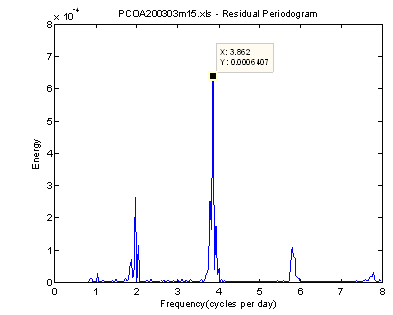
To gain experience with the residual periodogram, the user should first run a 29-day analysis with input file PCOA200303m15.xls (or PCOA200303m15.tsd), a data set containing currents in m/sec measured 15 m above bottom in Liverpool Bay on the eastern edge of the Irish Sea (Data supplied courtesy of the Proudman Oceanographic Laboratory, Liverpool Bay Coastal Observatory). After double clicking this file, examine the U,V scatter plot that appears and note the elliptical pattern of data points centered on the principal current axis. As previously shown in Fig. 1, the principal axis captures 98.6 percent of the total variance in U and V. Enter the principal axis heading of 96 degrees in the new axis / flood direction box, lock the heading and press ANALYZE with the high band periodogram enabled (radiobutton, frame on the right in Fig. 1). A U,V scatter plot will appear followed by the periodogram shown in Fig. 3.
Liverpool Bay is an example of a semidiurnal current system and the amplitudes of the principal diurnal constituents, O1 and K1, are small compared to the major semidiurnal constituents N2, M2 and S2. The periodogram that appears after pressing the ANALYZE button contains one large peak with an energy of 6.4 x 10⁻⁴ m2/sec2 per cpd at 3.862 cpd and two smaller ones at 1.966 and 5.793 cpd. Consulting the constituent frequency listbox, the first frequency is seen to be close to the quarterdiurnal constituent M4, the second falls midway between semidiurnal constituents LAM2 and L2 and the third is near the sixth-diurnal constituent M6. Use the MATLAB data cursor on the tool bar of the plot window and left click on the top of each peak to read its energy and frequency as shown in Fig. 3 below.
Run the analysis again with L2, M4 and M6 checked, noting their amplitudes in the listbox at the bottom of the page after the run. The amplitudes should read 0.032, 0.048 and 0.017 m/sec, respectively. These constituents should be kept as their amplitudes are reasonably large compared to N2, M2 and S2. The periodogram that will appear next for the second run now has five new peaks for the current residual at the next energy level moving down the scale.
After additional trial runs, constituents 2N2, K2, MN4, MS4 and 2MS6 also emerge as reasonable choices for inclusion in the tidal current model.
While adding constituents to the current prediction model, be certain to check the statistical parameters. The RMS error in the first stage at Liverpool Bay with O1, K1, N2, M2 and S2 is 0.077 m/sec and %R_Var is 97.04. These numbers change to 0.066 m/sec and 97.84% in the second stage and 0.061 m/sec and 98.19% in the third. In other words, of the 98.6% in total variance captured by the principal axis, the model can now explain 98.2 % of that variance (variance in Up) with the 13 selected constituents. A worksheet showing the constituent amplitudes and phases at each stage of the analysis is included in workbook PCOA200303m15.xls.
Example 2
Repeat the above steps with file RISFB200211sc.xls (Richmond, San Francisco Bay) for an example with surface current speed in knots and current direction in degrees clockwise from true north (Data supplied courtesy of the U.S. National Oceanic and Atmospheric Administration, Tides & Currents). Note that this file contains only 17 days of data as indicated in the series length data box. View the U,V scatter plot and enter a new flood heading of 331 degrees. After pressing ANALYZE, a 15-hour data gap will be apparent in the current plot on 7Nov2002 (Julian day 311). After entering ’311’ for a 3-day plot, this gap will be obvious (straight lines connecting the ends of the gap are an artifact of the MATLAB line plot routine and can be ignored). There are a number of smaller (6-min) gaps in this file as well but no time shifts.
The principal axis in this example accounts for 99.2 percent of the total U,V variance. Clearly very little information is given up after choosing this axis and the user may verify that the initial run with just the five basic constituents accounts for 96.84 percent of the Up variance. Turning next to the high band periodogram to seek more constituents, the large residual peak that appears at 2.928 cpd suggests MK3. After a trial, MK3 does not look promising in terms of both its amplitude and effect on % R_Var - or the energy peak itself. A trial with M3 yields much the same result. However the next constituent down the frequency scale, 2MK3, has significant amplitude and clearly reduces the residual peak at 2.928 cpd. Adding this constituent along with K2, MS4, M6 and 2MS6 in the third stage of the analysis increases the explained variance to 97.98 percent and reduces the RMS error to 0.176 knots, leaving very little energy in the residual. Checking predicted versus observed currents with the 3-day plot feature reveals a good match in most places considering that this series, like the Liverpool Bay example, is not without its share of ’noise’ in the peaks of the observed current.
Current speed histograms
Histograms provide information on the distribution of current speed. Mariners have long been accustomed to prediction tables that provide only the time, strength and direction of flood and ebb current maxima along with predictions of slack water times. Other professionals want to know about other aspects of the flow as well, including engineers who want to calculate fluid forces on structures, or who desire to exploit tidal power ( tidal currents) to generate electricity.
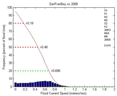
Histograms are provided on both the Analysis and the Prediction pages of TAP currents. On the Analysis page (Fig. 1), the user may select flood-and-ebb current speed distributions with frequencies given in percent of flood and ebb time. On the Predictions page (Fig. 4, Appendix B) users can make the same selections for monthly or yearly predictions with frequency given in either percent of time or in hours. In Analysis histograms, all current speeds are first reduced to their zero-mean value for the series; in Prediction histograms, current speeds include the mean, if any, transferred with the harmonic constants (see SAVING HARMONIC CONSTANTS).
Histograms generated during Analysis display both the observed and the predicted current speed distributions for the series being analyzed. The matching of these distributions can provide additional confirmation regarding choice of constituents. Analyze the RSFB file once more after checking the box the lower right corner of the page next to ’enable histogram’. TAPcurrents will then generate two pairs of histograms with cumulative curves for comparison of flood and ebb zero-mean current speed distributions, predicted versus observed. To aid the comparisons, three percentile points are shown on each curve at 20%, 50% and 80%. For example, the observed San Francisco Bay flood speeds equal or exceed 1.44 knots 20 percent of the time. For the constituents selected, 20 percent of all predicted flood currents also equal or exceed 1.44 knots over the same time interval at Richmond. The two remaining percentile levels are nearly in agreement although the cumulative curves are not identical at every point.
TAPcurrents Predictions

Clicking the Tidal Current Predictions button within the SMS menu Tools|Harmonic Analysis starts the GUI page that performs tidal current predictions. This will bring up the TIDAL CURRENTS: PREDICTION page. Clicking the selection button will allow the user to browse for tidal constants files created during Analysis; e.g., files for the Liverpool Bay and San Francisco Bay analyses described earlier. Opening the San Francisco Bay file will initiate the GUI shown in Fig. 4.
After opening a tidal constants file, the file name and analysis date will be displayed in the data box below the Select button. The symbols of the constituents used in deriving this file can be viewed by clicking on ’Tidal Constituents’ in the menu bar above the GUI page (not shown in Fig. 4). Select the month and year of the predictions wanted along with the other options displayed including units, plot grid, Local Standard time (LST) or Local Daylight Time (LDT). NOTE: It is assumed that observed current data files will not use daylight saving time. Pressing the large PREDICT button will then populate the calendar matrix at left with the days of the month and year selected. A daily, weekly or monthly plot of the predicted tidal current is displayed after the user presses the appropriate button.
Printing to a file
Checking the ’enable print to file’ box below PREDICT allows the user to print a series of 12-minute current predictions to a text file for the month and year selected. If the ’year’ button is also checked, predictions are printed for the year selected using a 30-minute prediction interval.
Predicted speed distributions
To display a histogram of the flood and ebb current speed distributions, depress either the ’histogram1(percent)’ or ’histogram2(hours)’ radiobutton. The histogram distributions include the mean current value appearing in the ’Mean Current’ databox on the Analysis page at the time the tidal constants file was saved (prior to saving, the user could have entered another value, including zero, in this box). If either histogram is selected along with ’print to file’ (or ’print to file’ and ’year’), a text file of the histogram values is printed in place of the serial current predictions.
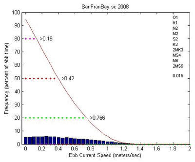
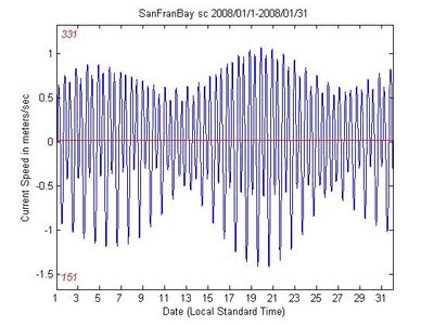
Examples of predicted flood and ebb speed distributions in San Francisco Bay (NOAA PORTS station near Richmond, California) for 2008 are shown in Fig. 5. It is apparent in these graphs that higher current speeds favor the ebb over the flood phase at this station. This result is directly related to a strong diurnal inequality in the peak ebb currents at Richmond as illustrated in Fig. 6.
Additional Information
Questions about this CHETN can be addressed Alex Sánchez at (601-634-2027), FAX (601-634-3433), or e-mail: [mailto: Alejandro.Sanchez@usace.army.mil Alejandro.Sanchez@usace.army.mil].
References
- Boon, J.D., 2004. Secrets of the Tide: Tide and Tidal Current analysis and Predictions, Storm surges and Sea Level Trends. Horwood Publishing, Chichester, U.K. 212 pp. Reprinted 2007.
- Cartwright, D.E., 2000. Tides: A scientific history. Cambridge University Press, 292pp.
- Pugh, David T., 2004. Changing Sea Levels: Effects of Tides, Weather and Climate. Cambridge University Press, 265 pp.