Visser: Difference between revisions
No edit summary |
m →Results |
||
| (33 intermediate revisions by one other user not shown) | |||
| Line 1: | Line 1: | ||
== Setup == | <big> | ||
__NOTOC__ | |||
== Experimental Setup == | |||
In 1991, Visser conducted eight laboratory experiments of monochromatic wave on a planar beach and collected measurements on waves, currents and water levels. The bathymetry consisted of a 1:10 slope for the first 1-m seaward distance, a 1:20 slope for the next 5-m distance, followed by a 5.9 m distance of flat bottom to the wave generator. Both experiments had incident wave heights of 0.078 m, peak periods of 1.02 sec and an incident wave angle of 15.4°. Experiment 4 was run over a concrete bed and experiment 7 was run of a thin 0.005-0.01 m layer of gravel grouted on the concrete floor. | In 1991, Visser conducted eight laboratory experiments of monochromatic wave on a planar beach and collected measurements on waves, currents and water levels. The bathymetry consisted of a 1:10 slope for the first 1-m seaward distance, a 1:20 slope for the next 5-m distance, followed by a 5.9 m distance of flat bottom to the wave generator. Both experiments had incident wave heights of 0.078 m, peak periods of 1.02 sec and an incident wave angle of 15.4°. Experiment 4 was run over a concrete bed and experiment 7 was run of a thin 0.005-0.01 m layer of gravel grouted on the concrete floor. | ||
'''Table 1. Experiment Regular Wave Conditions''' | |||
{| border="1" | {| border="1" | ||
! | ! Parameter !! Value | ||
|- | |- | ||
| Height | | Height, m || 0.08 | ||
|- | |- | ||
| Period | | Period, sec || 1.02 m | ||
|- | |- | ||
| | | Incident Angle,° || 15.4 | ||
|} | |} | ||
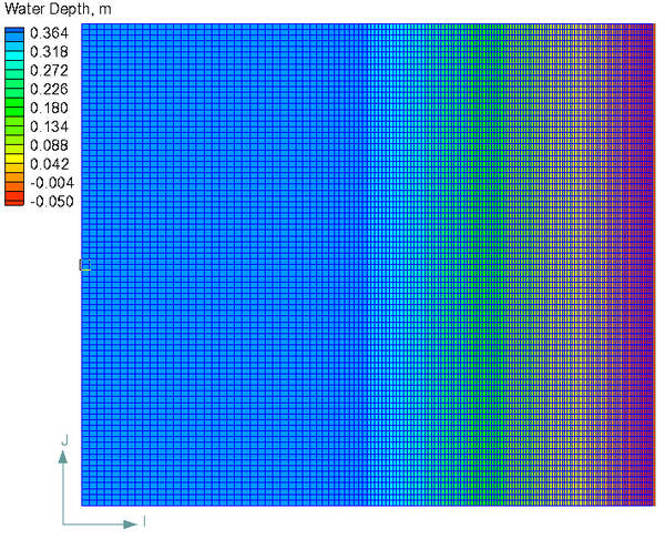
The computational grid (shown in Figure 1) consists of 84 rows and 147 columns with a constant grid resolution in the longshore direction of 0.15 and a variable grid resolution between 0.04 and 0.15 m in the cross-shore direction. A zero water level was forced at the offshore boundary. | == Model Setup == | ||
[[Image:Visser_Grid.png|thumb|right|600px|Computational Grid | alt=Computation Grid]] | |||
The computational grid (shown in Figure 1) consists of 84 rows and 147 columns with a constant grid resolution in the longshore direction of 0.15 and a variable grid resolution between 0.04 and 0.15 m in the cross-shore direction. A zero water level was forced at the offshore boundary. A summary of some of the simulation settings used for both experiment cases are shown in the tables below. | |||
'''Table 2. CMS-Flow Settings''' | |||
{| border="1" | |||
! Settings !! Value | |||
|- | |||
|Solution scheme || Implicit | |||
|- | |||
|Time Step || 60 sec | |||
|- | |||
| Wetting and Drying Depth || 0.006 m | |||
|- | |||
| Simulation Duration || 3 hr | |||
|- | |||
| Ramp Duration || 3 hr | |||
|- | |||
| Wave-current bottom friction || Fredsoe 1984 | |||
|} | |||
'''Table 3. CMS-Wave Settings''' | |||
{| border="1" | |||
! Settings !! Value | |||
|- | |||
| Wave Breaking || Battjes and Janssen | |||
|- | |||
| Bottom friction || Off | |||
|- | |||
| Steering Interval || 0.25 hr | |||
|} | |||
<br style="clear:both" /> | <br style="clear:both" /> | ||
== Results == | == Results == | ||
The | The calibration procedure consisted of first matching the wave profile by calibrating the location of the breaking wave height using the breaker index <math> \gamma </math>. The flow was then calibrated using the Manning's n coefficient and roller efficiency coefficient. The combined wave-current bottom friction was calculated based on Fredsoe 1984. Although this is not the default in CMS, it was choosen because of its strong theoritical backgroud compared to the default quadratic formula. Additional tests were run for comparison with the same settings except the roller model was turned off. | ||
'''Table 4. Calibration Parameters''' | |||
{| border="1" | |||
! Calibration Parameters !! Case 4 !! Case 7 !! Default | |||
|- | |||
| Breaker coefficient || 0.64 || 0.9 || 0.73 | |||
|- | |||
| Manning's n || 0.0115 || 0.018 || 0.025 | |||
|- | |||
| Roller efficiency coefficient || 0.8 || 0.8 || 1.0 | |||
|} | |||
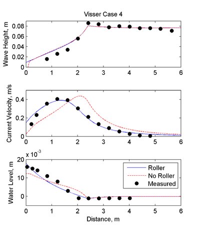
[[Image:Visser4.png|thumb|left|400px|Figure 1. Comparison of measured wave height, water levels and longshore currents for Visser Case 4.]] | |||
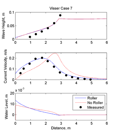
[[Image:Visser7.png|thumb|none|400px|Figure 2. Comparison of measured wave height and longshore currents for Visser Case 7 (Note: No water level measurements are available for this case).]] | |||
The goodness of fit statistics for both cases are shown in the table below | |||
'''Table 5. Goodness of fit statistics''' | |||
{|border="2" cellspacing="0" cellpadding="4" width="78%" | |||
|Statistic | |||
|align = "center" colspan = "3"|Case 4 | |||
|align = "center" colspan = "2"|Case 7 | |||
|- | |||
| | |||
|Wave Height, m | |||
|Longshore Current, m | |||
|Water level, m | |||
|Wave Height, m | |||
|Longshore Current, m | |||
|- | |||
|RMSE | |||
|0.0058 | |||
|0.0289 | |||
|0.030 | |||
|0.0093 | |||
|0.0186 | |||
|- | |||
|RMAE | |||
|0.0305 | |||
|0.0172 | |||
|0.006 | |||
|0.0359 | |||
|0.0649 | |||
|- | |||
|R<nowiki>^</nowiki>2 | |||
|0.992 | |||
|0.981 | |||
|0.980 | |||
|0.999 | |||
|0.982 | |||
|} | |||
* For a definition of the goodness of fit statistics see [[Statistics | Goodness of fit statistics]] | |||
<br style="clear:both" /> | <br style="clear:both" /> | ||
== References == | == References == | ||
*Visser, R. J. (1991) “Laboratory measurements of uniform longshore currents”. Coastal Engineering, 15, 563-593. | *Visser, R. J. (1991) “Laboratory measurements of uniform longshore currents”. Coastal Engineering, 15, 563-593. | ||
---- | ---- | ||
[[Test_Cases]] | [[Test_Cases | Test Cases]] | ||
[[CMS#Documentation_Portal | Documentation Portal]] | |||
Latest revision as of 16:42, 29 October 2010
Experimental Setup
In 1991, Visser conducted eight laboratory experiments of monochromatic wave on a planar beach and collected measurements on waves, currents and water levels. The bathymetry consisted of a 1:10 slope for the first 1-m seaward distance, a 1:20 slope for the next 5-m distance, followed by a 5.9 m distance of flat bottom to the wave generator. Both experiments had incident wave heights of 0.078 m, peak periods of 1.02 sec and an incident wave angle of 15.4°. Experiment 4 was run over a concrete bed and experiment 7 was run of a thin 0.005-0.01 m layer of gravel grouted on the concrete floor.
Table 1. Experiment Regular Wave Conditions
| Parameter | Value |
|---|---|
| Height, m | 0.08 |
| Period, sec | 1.02 m |
| Incident Angle,° | 15.4 |
Model Setup

The computational grid (shown in Figure 1) consists of 84 rows and 147 columns with a constant grid resolution in the longshore direction of 0.15 and a variable grid resolution between 0.04 and 0.15 m in the cross-shore direction. A zero water level was forced at the offshore boundary. A summary of some of the simulation settings used for both experiment cases are shown in the tables below.
Table 2. CMS-Flow Settings
| Settings | Value |
|---|---|
| Solution scheme | Implicit |
| Time Step | 60 sec |
| Wetting and Drying Depth | 0.006 m |
| Simulation Duration | 3 hr |
| Ramp Duration | 3 hr |
| Wave-current bottom friction | Fredsoe 1984 |
Table 3. CMS-Wave Settings
| Settings | Value |
|---|---|
| Wave Breaking | Battjes and Janssen |
| Bottom friction | Off |
| Steering Interval | 0.25 hr |
Results
The calibration procedure consisted of first matching the wave profile by calibrating the location of the breaking wave height using the breaker index . The flow was then calibrated using the Manning's n coefficient and roller efficiency coefficient. The combined wave-current bottom friction was calculated based on Fredsoe 1984. Although this is not the default in CMS, it was choosen because of its strong theoritical backgroud compared to the default quadratic formula. Additional tests were run for comparison with the same settings except the roller model was turned off.
Table 4. Calibration Parameters
| Calibration Parameters | Case 4 | Case 7 | Default |
|---|---|---|---|
| Breaker coefficient | 0.64 | 0.9 | 0.73 |
| Manning's n | 0.0115 | 0.018 | 0.025 |
| Roller efficiency coefficient | 0.8 | 0.8 | 1.0 |


The goodness of fit statistics for both cases are shown in the table below
Table 5. Goodness of fit statistics
| Statistic | Case 4 | Case 7 | |||
| Wave Height, m | Longshore Current, m | Water level, m | Wave Height, m | Longshore Current, m | |
| RMSE | 0.0058 | 0.0289 | 0.030 | 0.0093 | 0.0186 |
| RMAE | 0.0305 | 0.0172 | 0.006 | 0.0359 | 0.0649 |
| R^2 | 0.992 | 0.981 | 0.980 | 0.999 | 0.982 |
- For a definition of the goodness of fit statistics see Goodness of fit statistics
References
- Visser, R. J. (1991) “Laboratory measurements of uniform longshore currents”. Coastal Engineering, 15, 563-593.