Standing wave in a rectangular basin: Difference between revisions
No edit summary |
|||
| (4 intermediate revisions by the same user not shown) | |||
| Line 1: | Line 1: | ||
__NOTOC__ | |||
<font color=red>'''UNDER CONSTRUCTION'''</font> | |||
= Purpose = | = Purpose = | ||
The | The standing wave test case is useful for testing the model numerical dissipation for different temporal schemes. | ||
<br style="clear:both" /> | <br style="clear:both" /> | ||
= Problem = | = Problem = | ||
Assuming no Coriolis, bottom friction, advection, diffusion, and that the water elevation is much smaller than the water depth, the governing equations are given by | Assuming no Coriolis, bottom friction, advection, diffusion, and that the water elevation is much smaller than the water depth, the governing equations are given by | ||
| Line 27: | Line 31: | ||
where <math> k = m \pi / L </math> is the wave number (eigenvalue), with <math>m=1,2,...</math>, <math> \omega </math> is the wave frequency, and <math> T </math> is the wave (eigen) period given by | where <math> k = m \pi / L </math> is the wave number (eigenvalue), with <math>m=1,2,...</math>, <math> \omega </math> is the wave frequency, and <math> T </math> is the wave (eigen) period given by | ||
{{Equation|<math> T = \frac{2}{\sqrt{gh{m/L}^2}} </math>|5}} | {{Equation|<math> T = \frac{2}{\sqrt{gh{(m/L)}^2}} </math>|5}} | ||
When <math>m=1</math> the solution is referred to as the fundamental mode. The fundamental mode is the solution used here. | When <math>m=1</math> the solution is referred to as the fundamental mode. The fundamental mode is the solution used here. | ||
| Line 34: | Line 38: | ||
= Model Setup = | = Model Setup = | ||
[[File:Slosh_grid.png|right|thumb|400px| Figure 1. Computational grid for the | [[File:Slosh_grid.png|right|thumb|400px| Figure 1. Computational grid for the standing wave test case.]] | ||
The model domain is 1000 m long and 300 m wide. The computational grid is shown in Figure 1. The grid has a constant grid spacing of 100 m. | The model domain is 1000 m long and 300 m wide. The computational grid is shown in Figure 1. The grid has a constant grid spacing of 100 m. | ||
| Line 43: | Line 47: | ||
The model setup is summarized in Table 1. | The model setup is summarized in Table 1. | ||
Table 1. Summary of the model setup for the | |||
'''Table 1. Summary of the model setup for the standing wave test case.''' | |||
{| border="1" | {| border="1" | ||
! | ! Parameter !! Value | ||
|- | |- | ||
| Water depth || 10 m | | Water depth || 10 m | ||
| Line 71: | Line 76: | ||
= Results and Discussion = | = Results and Discussion = | ||
[[File:slosh_snaps.png|right|thumb|500px| Figure 2. Water level profiles at different times for the | [[File:slosh_snaps.png|right|thumb|500px| Figure 2. Water level profiles at different times for the standing wave test case calculated with the first and second order temporal schemes.]] | ||
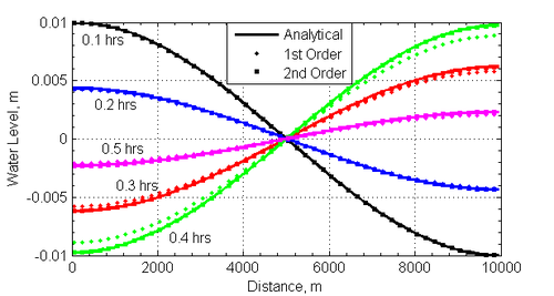
A time series of the water level at for both the 1st and 2nd order temporal schemes is shown in Figure 2. The 1st order temporal scheme shows significant numerical dissipation which reduces the amplitude of the standing wave. The 2nd order temporal scheme shows much less numerical dissipation and follows closely the analytical solution. | |||
[[File:slosh_snaps_2nd.png|right|thumb|500px| Figure 3. Water level profiles at different times for the | <br style="clear:both" /> | ||
[[File:slosh_snaps_2nd.png|right|thumb|500px| Figure 3. Water level profiles at different times for the standing wave test case calculated with the second order temporal scheme.]] | |||
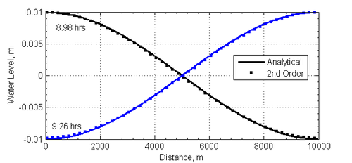
In order to demonstrate the low dissipation of the second order scheme, a snap shot of the water levels after approximately 16 and 16.5 wave cycles is shown for the second order temporal scheme in Figure 3. | |||
<br style="clear:both" /> | |||
[[File:slosh_timeseries.png|right|thumb|500px| Figure 4. Water level time series calculated at x=L using the first and second order temporal schemes. ]] | [[File:slosh_timeseries.png|right|thumb|500px| Figure 4. Water level time series calculated at x=L using the first and second order temporal schemes. ]] | ||
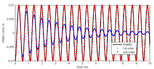
The difference in numerical dissipation between 1st and 2nd order temporal schemes can be appreciated in Figure 4 which shows a time series of the water levels calculated at <math> x = L </math>. In the case of the 1st order scheme, the wave amplitude is reduced by approximately half within 4 wave cycles, while the 2nd order schemes maintains the same wave amplitude for the duration of the simulation. | |||
<br style="clear:both" /> | |||
It is noted that there is a small inconsistency between the problem governing equations and the model governing equations. The numerical model solves the shallow water equations in conservative form and does not assume that the wave amplitude is small relative to the water depth. However, as long as the the wave amplitude is specified such that it is much small than the water depth, the model governing equations are approximately equivalent to equations (1) and (2). The goodness-of-fit statistics for the time series comparison are shown in Table 2. | |||
<br style="clear:both" /> | <br style="clear:both" /> | ||
'''Table 2. Goodness-of-fit statistics* for standing wave test case for the 1st and 2nd order temporal schemes. The normalization was done with the wave amplitude = 1 cm.''' | |||
{|border="1" | |||
|Statistic || 1st Order || 2nd Order | |||
|- | |||
|NRMSE || 0.5223 || 0.0560 | |||
|- | |||
|NMAE || 0.4406 || 0.0430 | |||
|- | |||
|R^2|| 0.5847 || 0.9937 | |||
|} | |||
* For a definition of the goodness of fit statistics see [[Statistics | Goodness of fit statistics]]. | |||
<br style="clear:both" /> | |||
= References = | = References = | ||
* Ferziger, J. H., and Peric, M., 1997. Computational Methods for Fluid Dynamics, Springer-Verlag, Berlin/New York, 423 p. | * Ferziger, J. H., and Peric, M., 1997. Computational Methods for Fluid Dynamics, Springer-Verlag, Berlin/New York, 423 p. | ||
Latest revision as of 20:14, 18 April 2013
UNDER CONSTRUCTION
Purpose
The standing wave test case is useful for testing the model numerical dissipation for different temporal schemes.
Problem
Assuming no Coriolis, bottom friction, advection, diffusion, and that the water elevation is much smaller than the water depth, the governing equations are given by
| (1) |
| (2) |
where
- = time [s]
- = horizontal coordinate [m]
- = current velocity [m/s]
- = water depth [m]
- = water level with respect to the Still Water Level (SWL) [m]
Eliminating the velocity from both equations leads to the classical wave equation
| (3) |
Given a closed rectangular basin of length and width , the following solution can be found for simple harmonic motion (Lamb 1945)
| (4) |
where is the wave number (eigenvalue), with , is the wave frequency, and is the wave (eigen) period given by
| (5) |
When the solution is referred to as the fundamental mode. The fundamental mode is the solution used here.
Model Setup

The model domain is 1000 m long and 300 m wide. The computational grid is shown in Figure 1. The grid has a constant grid spacing of 100 m.
The temporal tem is approximated by
| (6) |
where is a weighting factor between 0 and 1. For = 0, the scheme reduces to the first-order backward Euler scheme, and with = 1, the scheme reduces to the second-order backward scheme (Ferziger and Peric 1997).
The model setup is summarized in Table 1.
Table 1. Summary of the model setup for the standing wave test case.
| Parameter | Value |
|---|---|
| Water depth | 10 m |
| Wave amplitude | 1 cm |
| Time step | 18 s |
| Simulation duration | 10 hrs |
| Ramp period | 0 s |
| Grid resolution | 100 m |
| Advection | Off |
| Diffusion | Off |
| Bottom friction | Off |
| Temporal scheme | 1st and 2nd order |
Results and Discussion

A time series of the water level at for both the 1st and 2nd order temporal schemes is shown in Figure 2. The 1st order temporal scheme shows significant numerical dissipation which reduces the amplitude of the standing wave. The 2nd order temporal scheme shows much less numerical dissipation and follows closely the analytical solution.

In order to demonstrate the low dissipation of the second order scheme, a snap shot of the water levels after approximately 16 and 16.5 wave cycles is shown for the second order temporal scheme in Figure 3.

The difference in numerical dissipation between 1st and 2nd order temporal schemes can be appreciated in Figure 4 which shows a time series of the water levels calculated at . In the case of the 1st order scheme, the wave amplitude is reduced by approximately half within 4 wave cycles, while the 2nd order schemes maintains the same wave amplitude for the duration of the simulation.
It is noted that there is a small inconsistency between the problem governing equations and the model governing equations. The numerical model solves the shallow water equations in conservative form and does not assume that the wave amplitude is small relative to the water depth. However, as long as the the wave amplitude is specified such that it is much small than the water depth, the model governing equations are approximately equivalent to equations (1) and (2). The goodness-of-fit statistics for the time series comparison are shown in Table 2.
Table 2. Goodness-of-fit statistics* for standing wave test case for the 1st and 2nd order temporal schemes. The normalization was done with the wave amplitude = 1 cm.
| Statistic | 1st Order | 2nd Order |
| NRMSE | 0.5223 | 0.0560 |
| NMAE | 0.4406 | 0.0430 |
| R^2 | 0.5847 | 0.9937 |
- For a definition of the goodness of fit statistics see Goodness of fit statistics.
References
- Ferziger, J. H., and Peric, M., 1997. Computational Methods for Fluid Dynamics, Springer-Verlag, Berlin/New York, 423 p.
- Lamb, H., 1945. Hydrodynamics, 6th ed., Dover, New York, 738 p.
- Mei, C.C., 1992. The Applied Dynamics of Ocean Surface Waves, World Scientific, London, 740 p.