Standing wave in a rectangular basin

Purpose

The sloshing test case is useful for testing the model numerical dissipation for different temporal schemes. It is noted that the analytical solution uses the linear shallow water equations which assume that the wave amplitude is much smaller than the water depth.

Problem

Assuming no Coriolis, bottom friction, advection, diffusion, and that the water elevation, is much smaller than the water depth, the governing equations are given by

${\frac {\partial \eta }{\partial t}}+h{\frac {\partial U}{\partial x}}=0$

(1)

${\frac {\partial U}{\partial x}}=-gfrac{\partial \eta }{\partial x}$

(2)

where

$t$ = time [s]

$x$ = horizontal coordinate [m]

$U$ = current velocity [m/s]

$h$ = water depth [m]

$\eta$ = water level with respect to the Still Water Level (SWL) [m]

Eliminating the velocity from both equations leads to the classical wave equation (4) If the waves are sinusoidal of the form (5) (6) where , is the wave frequency, and and are the current velocity and water level amplitudes, respectively. Substituting the above expressions into the wave equation leads to the Helmholtz equation (7) where is the wave number with is the wave celerity. At the lateral boundaries the flux is set to zero (8) where unit vector normal to the boundary. Given a rectangular basin of length and width , the eigensolutions are found by separation of variables (9) where , is the wave frequency, and is the eigen (wave) period. The wave period is given by (10) The eigenvalues (wavenumbers) are given by (11)

Model Setup

Figure 1. Computational grid for the sloshing test case.

The model domain is 1000 m long and 300 m wide. The computational grid is shown in Figure 1. The grid has a constant grid spacing of 100 m.

The temporal tem is approximated by (11) where is a weighting factor between 0 and 1. For = 0, the scheme reduces to the first-order backward Euler scheme, and with = 1, the scheme reduces to the second-order backward scheme (Ferziger and Peric 1997).

The model setup is summarized in Table 1. Table 1. Summary of the model setup for the sloshing test case. Model Parameter Value Water depth 10 m Wave amplitude 1 cm Time step 18 s Simulation duration 10 hrs Ramp period 0 s Grid resolution 100 m Advection Off Diffusion Off Bottom friction Off Temporal scheme 1st and 2nd order

Results

Figure 2. Water level profiles at different times for the sloshing test case calculated with the first and second order temporal schemes.

Figure 3. Water level profiles at different times for the sloshing test case calculated with the second order temporal scheme.

Figure 4. Water level time series calculated at x=L using the first and second order temporal schemes.

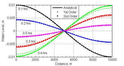
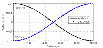
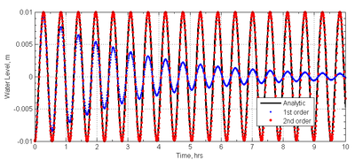
A time series of the water level at for both the 1st and 2nd order temporal schemes is shown in Figure 4. The 1st order temporal scheme shows significant numerical dissipation which reduces the amplitude of the standing wave. The 2nd order temporal scheme shows much less numerical dissipation and agrees much better with the analytical solution.

References

• Ferziger, J. H., and Peric, M., 1997. Computational Methods for Fluid Dynamics, Springer-Verlag, Berlin/New York, 423 p.
• Lamb, H., 1945. Hydrodynamics, 6th ed., Dover, New York, 738 p.
• Mei, C.C., 1992. The Applied Dynamics of Ocean Surface Waves, World Scientific, London, 740 p.

---

Test Cases Documentation Portal