Long-wave Runup: Difference between revisions
Jump to navigation
Jump to search
No edit summary |
|||
| Line 2: | Line 2: | ||
__NOTOC__ | __NOTOC__ | ||
<font color=red>'''UNDER CONSTRUCTION'''</font> | <font color=red>'''UNDER CONSTRUCTION'''</font> | ||
== | == Overview == | ||
where <math>\eta</math> is the water surface elevation, <math>\rho</math> is the water density, <math>\rho_a</math> is the air density, <math>g</math> is the gravitational acceleration, <math>W</math> is the wind speed, <math>h</math> is the water depth, and <math>C</math> is a constant of integration. | |||
== Initial Condition == | |||
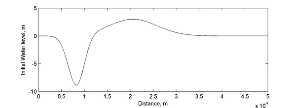
[[Image:Long-wave_Runup_Initial_Water_Level.png|thumb|left|600px| Figure 1. Computed water surface elevation for the irregular domain with constant water depth.]] | |||
<br style="clear:both" /> | |||
== Model Setup == | == Model Setup == | ||
A computational grid with constant water depth of 5 m and irregular boundaries is used in order to test the model performance. The computational grid has 60 columns and 70 rows and a constant resolution of 500 m. | A computational grid with constant water depth of 5 m and irregular boundaries is used in order to test the model performance. The computational grid has 60 columns and 70 rows and a constant resolution of 500 m. | ||
== Results == | == Results == | ||
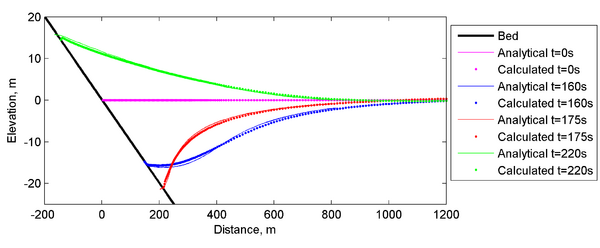
[[Image:Long-wave_Runup_Water_Level. | [[Image:Long-wave_Runup_Water_Level.png|thumb|none|600px| Figure 2. Comparison of computed water surface elevation to the analytical solution for an irregular basin with constant depth.]] | ||
<br style="clear:both" /> | <br style="clear:both" /> | ||
== References == | == References == | ||
Revision as of 00:01, 14 January 2011
UNDER CONSTRUCTION
Overview
where is the water surface elevation, is the water density, is the air density, is the gravitational acceleration, is the wind speed, is the water depth, and is a constant of integration.
Initial Condition

Model Setup
A computational grid with constant water depth of 5 m and irregular boundaries is used in order to test the model performance. The computational grid has 60 columns and 70 rows and a constant resolution of 500 m.
Results
