3-Numerical Methods

3 Numerical Methods

Overview

CMS-Flow has both implicit and explicit solution schemes. The explicit solver is designed for dynamic problems with extensive wetting and drying that require small computational time steps, while the implicit solver is intended for simulating tidal- and wave-induced circulation at tidal inlets, navigation channels, and adjacent beaches. A detailed description of the numerical formulation of the explicit solver of CMS-Flow can be found in Buttolph et al. (2006) and is not repeated here. The sections below specifically refer to the implicit solver of CMS-Flow.

The implicit solver uses the SIMPLEC algorithm (Van Doormal and Raithby 1984) on a non-staggered grid to handle the coupling of water level and velocity. Primary variables u-, v-velocity, and water level are stored on the same set of grid points, and fluxes at cell faces are determined using a Rhie and Chow (1983) type momentum interpolation method (Wu et al. 2011). The explicit solver uses a staggered grid with velocities at the cell faces and the water levels and water depths at the cell centers (Buttolph et al. 2006a). CMS-Flow also calculates salinity, sediment transport, and morphology change.

CMS-Flow Computational Grid

The implicit version of CMS-Flow uses a generic Cartesian grid which can be regular, nonuniform, or locally refined by splitting a cell into four subcells. Three requirements are necessary for the input grid:

1. Cells must have a rectangular shape. Irregularly shaped cells are not allowed.

2. Cells may have a total of four to six neighboring cells (faces).

3. Only two neighboring cells are allowed in the same direction (i.e. North, South, East, West).

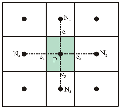
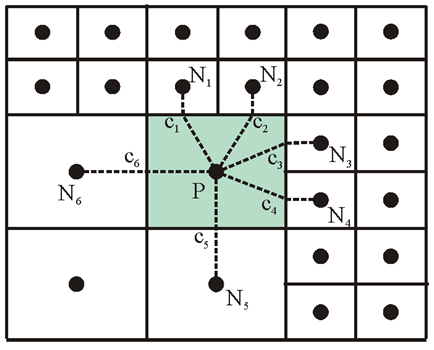
Mesh refinement can be achieved either by locally decreasing the grid spacing (nonuniform Cartesian grid) as shown in the left panel of Figure 3.1 or by subdividing or splitting a cell into multiple cells as shown in the right panel of Figure 3.1. The refined mesh can be further refined and split in multiple levels, as needed. This mesh is referred to here as a telescoping mesh.

Figure 3.1. Examples of a Cartesian grids allowed in CMS: Stretched Cartesian (left) and telescoping grid (right)

One important aspect of incompressible flow models is the location of primary variables: velocity and pressure (water level). On a staggered grid, the pressure (water level) is located at the center of cells and the u- and v-velocities are located along the faces of cells (Harlow and Welsh 1965; Patankar 1980). On a non-staggered grid, all of the primary variables are located at the center of cells. A staggered grid can more easily eliminate the checkerboard oscillations when compared to a non-staggered grid; however, a non-staggered grid involves a simpler source code and can minimize the number of coefficients that must be computed and stored during a simulation because many of the terms in the equations are approximately equal. In particular, a staggered grid is more complicated when handling the interface between coarse and fine cells where five- or six-face control volumes are used. Therefore, a non-staggered (collocated) grid approach is adopted for CMS-Flow, with a Rhie and Chow (1983) momentum interpolation technique used to eliminate the checkerboard oscillations. Figure 3.1 shows the location of primary variables and the 5- and 7-point stencils (computational molecule) used in the calculations for CMS-Flow.

The data structure for a grid can be approached in three ways: 1) block-structured, 2) hierarchical tree, and 3) unstructured. The block-structured approach divides the domain into multiple blocks and each block is treated as structured. A special treatment is applied between blocks to ensure mass and momentum balance using this approach. The hierarchical tree approach is memory intensive and requires parent-child relationships and a tree traverse to determine mesh connectivity. For the unstructured approach, all cells are numbered in a one-dimensional sequence and tables are used to determine the connectivity of neighboring cells. Among these three approaches, the unstructured approach is the most simple and is therefore applied in CMS-Flow.

Computational cells are numbered in an unstructured manner via a 1-D index array. Inactive cells (permanently dry) are not included in the 1-D index array to save memory and computational time. All active computa-tional nodes are numbered sequentially. For convenience with handling boundary conditions, each boundary cell has a neighboring ghost cell outside of the computational domain. Each ghost cell corresponds to a boundary face of the boundary cell. The ghost cells are stored at the end of the 1-D index array.

General Transport Equation

In order to avoid redundant derivations of discretized equations, discretization of a general transport equation is outlined and described below. All of the governing equations are some form of this transport equation; therefore, the same discretization may be applied to all of the governing equations. The general transport equation is given by

$\underbrace {\frac {\partial (h\phi )}{\partial t}} _{\text{Temporal Term}}+\underbrace {\frac {\partial (hV_{j}\phi )}{\partial x_{j}}} _{\text{Advection Term}}=\underbrace {{\frac {\partial }{\partial x_{j}}}\left(\Gamma h{\frac {\partial \phi }{\partial x_{j}}}\right)} _{\text{Diffusion Term}}+\underbrace {S_{\phi }} _{\text{Source Term}}$

(3-1)

where $\phi$ is a general scalar, t is time, h is the total water depth, $V_{j}$ is the transport velocity, $\Gamma$ is the diffusion coefficient for $\phi$ , and $S_{\phi }$ includes all remaining terms. Note that in the case of the continuity and momentum equations, $\phi$ is equal to 1 and $U_{j}$ , respectively.

Spatial Discretization

A control-volume technique is used in which the governing equations are integrated over a control volume to obtain an algebraic equation that can be solved numerically. Integration of Equation (3-1) over a control volume yields:

$\int _{A}{\frac {\partial (h\phi )}{\partial t}}dA+\int _{A}{\frac {\partial }{\partial x_{j}}}\left(hV_{j}\phi -\Gamma h{\frac {\partial \phi }{\partial x_{j}}}\right)dA=\int _{A}S_{\phi }dA$

(3-2)

${\frac {\partial (h_{P}\phi _{P})}{\partial t}}\Delta A_{P}+\int _{L}h[({\hat {n_{i}}}V_{i})\phi -\Gamma ({\hat {n_{i}}}\bigtriangledown _{i}\phi )]dL=S_{\phi }\Delta A_{p}$

(3-3)

${\frac {\partial (h_{P}\phi _{P})}{\partial t}}\Delta A_{P}+\sum _{f}h_{f}\left[U_{f}\phi _{f}-\Gamma _{f}(\bigtriangledown _{\perp }\phi )_{f}\right]\Delta l_{f}=S_{\phi }\Delta A_{p}$

(3-4)

where

${\hat {n_{i}}}=({\hat {n_{1}}},{\hat {n_{2}}})$ = outward unit vector normal to cell face f

$V_{f}=({\hat {n_{i}}}V_{i})_{f}$ = outward cell face velocity

h_f = linearly interpolated total water depth at the cell face f

$(\bigtriangledown _{\perp }\phi )_{f}=({\hat {n_{i}}}\bigtriangledown _{i}\phi )_{f}$ is the outward normal gradient of $\phi$ at cell face f

The above equations, the Green-Gauss Theorem has been used to convert the area integral to a boundary integral. The symbol () indicates the cell face linear interpolation operator. The cell face velocity,$V_{f}$ , is calculated using a momentum interpolation method similar to that of Rhie and Chow (1983) and is described in a subsequent section.

Temporal Discretization

The general transport equation is rewritten as

$\int {\frac {\partial (h\phi )}{\partial t}}dt=\int Fdt$

(3-5)

where F includes all the remaining terms, such as …. For stability and efficiency, a fully implicit time-stepping scheme is used in the form

${\frac {(1+0.50\theta )h^{n+1}\phi ^{n+1}-(1+\theta )h^{n}\phi ^{n}+0.5\theta h^{n-1}\phi ^{n-1}}{\Delta t}}=F^{n+1}$

(3-6)

where $\theta$ is a weighting factor between 0 and 1. For $\theta =0$, the scheme reduces to the first-order backward Euler scheme, and with $\theta =1$, the scheme reduces to the second-order backward scheme (Ferziger and Peric 1997). The superscripts indicate the time step levels, with n+1 being the current timestep and n being the previous timestep.

Cell-face interpolation operator

The general formula for estimating the cell-face interpolation operator (?) value of $\phi _{f}$ is given by

$\phi _{f}=f_{\perp }\phi _{N}+(1-f_{\perp })\phi _{P}+f_{\perp }(r_{\Box }\bigtriangledown _{\Box }\phi )_{N}+(1-f_{\perp })(r_{\Box }\bigtriangledown _{\Box }\phi )_{P}$

(3-7)

where $f_{\perp }$ is a linear interpolation factor, $\bigtriangledown _{\Box }$ is the gradient operator in the direction parallel to face f, and $r_{\Box }$ is the distance from the cell center to the ghost point O parallel to the cell face f (see Figure 3.2).

Figure 3.2. Schematic showing two types of refined cells.

By definition,$\Box =2\mid {\hat {n_{1}}}\mid +1\mid {\hat {n_{2}}}\mid$ and $\perp =1\mid {\hat {n_{1}}}\mid +2\mid {\hat {n_{2}}}\mid$ . Note that for neighboring cells without any refinement, $r_{\Box }$ is equal to zero and the above equation is consistent with non-refined cell faces. The linear interpolation factor is defined as

$f_{\perp }={\frac {x_{\perp ,f}-x_{\perp ,P}}{x_{\perp N}-x_{\perp ,P}}}={\frac {\Delta x_{\perp ,P}}{\Delta x_{\perp ,P}+\Delta x_{\perp ,N}}}$

(3-8)

where $x_{\perp ,f}$ is the coordinate of f perpendicular to the face and $\Delta x_{\perp }$ is the cell dimension perpendicular to the face f.

Advection Schemes

Hybrid Scheme

The hybrid scheme is a composed of a first-order upwind scheme and a second-order central difference scheme. When the Peclet number, $P_{f}$, is larger than 2, the first-order upwind scheme is used; otherwise, the second-order central difference scheme is used:

$\phi _{f}=\left\{{\begin{aligned}&(\phi _{D}+\phi _{c})/2&for\mid P_{f}\mid <2\\&\phi _{c}&for\mid P_{f}\mid >2\end{aligned}}\right.$

(3-9)

where the subscripts D and C indicate the first downstream and first upstream nodes and $P_{f}=U_{f}|\delta _{\perp }|/{\bar {\Gamma _{f}}}$ is the Peclet number at the cell face in which $|\delta _{\perp }|=|x_{\perp ,N}-x_{\perp ,P}|$ .

Exponential Scheme

The exponential scheme interpolates the face value using an exact solution to the 1-D steady advection-diffusion equation:

${\frac {\phi _{f}-\phi _{0}}{\phi _{L}-\phi _{0}}}={\frac {exp(P_{f}x_{f}/|\delta _{\perp }|)-1}{exp(P_{f})-1}}$

(3-10)

where $\phi _{0}=\phi |_{x=0},\phi _{L}=\phi |_{x=L}$ . The exponential scheme has automatic upwinding and is stable, but is usually less than second order.

Hybrid Linear/Parabolic Scheme

The Hybrid Linear/Parabolic Approximation scheme of Zhu (1991) may be written as

$\phi _{f}=\left\{{\begin{aligned}&\phi _{c}+(\phi _{d}-\phi _{c}){\hat {\phi _{c}}}&for0\leq {\hat {\phi _{c}}}\leq 1\\&\phi _{c}&otherwise\end{aligned}}\right.$

(3-11)

where the subscripts D, C and indicate the first downstream and first and second upstream cells, respectively. The normalized variable, ${\hat {\phi _{c}}}$ , is determined based on the formulation of Jasak et al. (1999)

${\hat {\phi _{c}}}={\frac {\phi _{C}-\phi _{U}}{\phi _{D}-\phi _{U}}}=1-{\frac {\phi _{D}-\phi _{C}}{2(\bigtriangledown _{\perp }\phi )_{C}\delta _{\perp ,C}}}$

(3-12)

where $\sigma _{\perp ,C}=x_{\perp ,D}-x_{\perp ,C}$ . The Hybrid Linear/Parabolic Approximation scheme is second order.

Cell-face gradient operator

A linearly exact second-order approximation for the normal gradient at cell face f is calculated using the auxiliary node concept of Ferziger and Peric (1997)

$(\bigtriangledown _{\perp }\phi )_{f}={\frac {\phi _{N}-\phi _{P}+(r_{\Box }\bigtriangledown _{B}ox\phi )_{N}-(r_{\Box }\bigtriangledown _{\Box }\phi )_{p}}{|\sigma _{\perp }|}}$

(3-13)

where the subscripts P and N refer to two neighboring cells, $|\sigma _{\perp }|=|x_{\perp ,N}-x_{\perp ,P}|$ is the distance between cells P and N, normal to the cell face (see Figure 3.2), and $\bigtriangledown _{\Box }$ is the gradient operator in the direction par-allel to face f. Ham et al. (2002) compared the auxiliary node formulation to the fully-unstructured discretization proposed by Zwart et al. (1998) for the viscous terms and found that the auxiliary node formulation is significantly more stable.

Cell-centered gradient operator

The cell-centered gradient operator is calculated using the Green-Gauss Theorem as

$\int _{A}\bigtriangledown _{i}\phi dA=\sum _{f}{\hat {n_{i}}}\phi _{f}\Delta l_{f}$

(3-14)

Equation 3-14 above is second order and conservative for regular and nonuniform grids.

Reconstruction, Monotonicity, and Slope Limiters

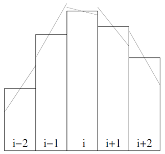
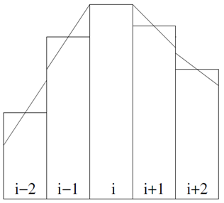
Given a conservative average value ${\bar {\phi }}$ within a cell, a linear reconstruction of the variable is used within that cell. This can be expressed as

$\phi ={\hat {\phi }}+{\overrightarrow {r}}\cdot \bigtriangledown _{\phi }$

(3-15)

The reconstruction is conservative in the sense that $\int _{\omega }\phi dA$ . If the reconstruction satisfies the local maximum principle

$min(\phi -{\bar {\phi }},0)\leq {\overrightarrow {r}}\cdot \bigtriangledown _{\phi }\leq max(\phi -{\hat {\phi }},0)$

(3-16)

then no new extrema are created within the cell and the solution is monotonic. Figure x shows two examples of linear reconstruction with and without slope limiters to ensure monotonicity.

then no new extrema are created within the cell and the solution is monotonic. Figure x shows two examples of linear reconstruction with and without slope limiters to ensure monotonicity.

Figure 3.3. Schematics showing examples of non-limited (a) and limited (b) linear reconstructions.

For non-telescoping grids, the slope limiter is calculated as

$\Phi (r)=\left\{{\begin{aligned}&{\frac {4r}{(r+1)^{2}}}\quad vanLeer(1979)\\&{\frac {2r}{(r^{2}+1)}}\quad vanAlbada1979\\&min\left(1,{\frac {4}{r+1}},{\frac {4r}{r+1}}\right)\quad MUSCL(vanLeer1979)\end{aligned}}\right.$

(3-17)

where r is the ratio between two consecutive slopes

$r={\frac {(\phi _{i+1}-\phi _{i})(x_{i}-x_{i-1})}{(x_{i+1}-x_{i})(\phi _{i}-\phi _{i-1})}}$

(3-18)

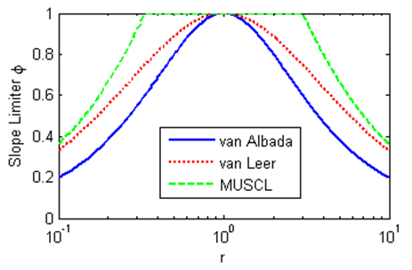
Here the second-order van Leer (1979) limiter is used because of its smoothness. Figure X shows a comparison of three different common limiters. The slope limiter is applied in each direction separately.

Figure 3.4. Comparison of three different slope limiters.

For joint cells, the standard slope limiters described above are difficult to implement because of the difficulty in defining forward and backward differences. Therefore for joint cells, a variation of the Limited Central Difference (LCD) slope limiting procedure of Hubbard (1999)

Equation{{|$\Phi _{f}=\left\{{\begin{aligned}&{\frac {max(\phi _{N}-\phi _{P},0)}{{\overrightarrow {r}}_{Pf}\cdot \bigtriangledown \phi _{p}}}&for{\overrightarrow {r}}_{Pf}\cdot \bigtriangledown \phi _{P}>max(\phi _{N}-\phi _{P},0)\\&{\frac {min(\phi _{N}-\phi _{P},0)}{{\overrightarrow {r}}_{Pf}\cdot \bigtriangledown \phi _{P}}}&for{\overrightarrow {r}}_{Pf}\cdot \bigtriangledown \phi _{P}<min(\phi _{N}-\phi _{P},0)\\&1&otherwise\\\end{aligned}}\right.$|3-19}}

where ${\overrightarrow {r}}_{pf}={\hat {x_{f}}}-{\hat {x_{p}}}$. In the procedure outlined by Hubbard (1999), a scalar limiter is then calculated as $\Phi =min(\Phi _{f})$ . For telescoping grids a directional limiter can be calculated as $\Phi _{i}=min(\Phi _{f})$ , which is less dissipative. Look at this again

Source/sink term

The source/sink term is linearized as (Patankar 1980)

$\int _{A}SdA=(S^{C}+S^{P}\phi )\Delta A_{p}$(3-20)

where $\Delta A_{p}$ is the cell area, and $S=S^{C}+S^{P}\phi$ is approximated as the cell-average source/sink term. The coefficient $S^{P}$ is required to be non-positive for stability.

Assembly of Algebraic Equations

Assembly refers to the process of combining terms to create a linear sys-tem of algebraic equations. The algebraic equation for each cell is obtained by first combining or assembling all of the terms. Then, the continuity equation is multiplied by $\phi _{p}^{n+1}$ and is subtracted from the transport equation. The resulting discretized equation for cell P is

$a_{P}\phi _{P}^{n+1}=\sum _{N}a_{N}\phi _{N}^{n+1}+b_{\phi }$(3-21)

where the subscript N refers to the neighboring cell sharing cell face, $a_{P}$ and $a_{N}$ are linear coefficients for $\phi _{P}^{n+1}$ and $\phi _{N}^{n+1}$ . The last term, $b_{\phi }$ , con-tains all the remaining terms (such as…name the specific terms here). Applying a similar equation for all of the internal cells of a grid results in a system of algebraic equations. This set of equations are referred to as the discretized governing equations.

Implicit Relaxation

Under-relaxation stabilizes the convergence of the outer non-linear iteration loop by introducing a relaxation parameter in the discretized equations (Patankar 1980) as

${\frac {a_{P}}{\alpha _{\phi }}}\phi _{P}^{n+1}=\sum _{N}a_{N}\phi _{N}^{n+1}+b_{\phi }+{\frac {1-\alpha _{\phi }}{\alpha _{\phi }}}a_{P}\phi _{P}^{m}$(3-22)

where $\alpha _{\phi }$ is an under-relaxation parameter and $\phi ^{m}$ is the value of $\phi$ from the previous iteration. An effect of under-relaxation is to make the coefficient matrix more diagonally dominant.

Iterative Solvers

The selection of an iterative solver is one key issue concerning the overall per-formance of the model. CMS has three iteration solvers available and they are described in more detail below: 1) GMRES variation, 2) BiCGStab, and 3) Gauss-Seidel. The default iterative solver for CMS is a variation of the GMRES (\underline{G}eneralized \underline{M}inimum \underline{RES}idual) method (Saad 1993) and is used to solve the algebraic equations. The original GMRES method (Saad and Schultz 1986) utilizes the Arnoldi process to reduce the coefficient matrix to the Hessenburg form and minimizes the norm of the residual vector over a Krylov subspace at each iterative step. The variation of the GMRES method recommended by Saad (1993) allows changes in preconditioning at every iteration step. An Incomplete LU Factorization (ILUT; Saad, 1994) is used as the preconditioner to speed-up convergence. The GMRES solver is applicable to symmetric and non-symmetric matrices and leads to the smallest residual for a fixed number of iterations. However, the memory requirements and computational costs become increasingly expensive for larger systems.

The BiCGStab (BiConjugate Gradient Stabilized) iterative solver is also a Krylov subspace solver and is applicable to symmetric and non-symmetrix matrices (Saad 1996). BiCGStab also uses ILUT as a preconditioner (Saad 1994). The BiCGStab method can be viewed as a combination of the standard Biconjugate Gradient solver where each iterative step is followed by a restarted GMRES iterative step. One advantage of the BiCGStab iterative solver is that the memory requirements are constant for each iteration and there are less computational costs when compared to the GMRES method (for GMRES restart numbers larger than 4).

The simplest iterative solver implemented in CMS is the point-implict Gauss-Seidel solver. This method may be applied in CMS with or without Succesive-Over-Relaxation to speed-up convergence (Patankar 1980). Even though the Gauss-Seidel method requires more iterations for convergence, the overall efficiency may be higher than the GMRES and BiCGStab because each itera-tion is computationally inexpensive and the code is parallelized. However, the GMRES and BiCGStab methods are more robust and perform better for large time steps.

Convergence and Time-Stepping

During the iterative solution process, error is calculated and used to de-termine if a solution has converged, diverged, or stalled at an error below a set tolerance threshold. Anestimate of the error in solving the general algebraic equation is given by

$r_{p}={\frac {1}{a_{p}}}\left(\sum _{N}a_{N}\phi _{N}^{n+1}-a_{P}\phi _{P}^{n+1}+b_{\phi }\right)$(3-23)

Statistics (such as…) can be defined based on normalized errors. For ex-ample, the $l^{2}$-norm is given by

$\|r\|_{2}={\sqrt {\sum _{cellsP}r_{P}^{2}}}$(3-24)

Since this value depends on the total number of cells, the final statistic (referred to as the residual) that is used for estimating the model convergence is obtained by dividing the norm by the number of cells

$R^{m}={\frac {\|r\|_{2}}{\sqrt {N_{c}}}}$(3-25)

$R^{m}$ is referred to as the “normalized residual error” and the superscript refers to the iteration number. $R^{m}$is calculated for each variable that is solved at each iteration step of the solution process. Each equation has default maximum tolerances for determining if the solution has converged, diverged, or stalled. The maximum number of iterations that is imposed is set equal to M. A minimum of 5 iterations are required for the hydrodynamic equations, and a minimum of M/2 iterations are required for the sediment transport equations. Table 3-1 lists the default criteria to determine whether the iterative solution procedure has converged, diverged, or requires a reduced time step.

Table 3-1. Default criteria to determine whether the iterative solution procedure has converged, diverged, or requires a reduced time step.

Variable	Converged	Diverged	Reduce Time Step
Current velocity, m/s	If Rm < 1x10-7 or | Rm-Rm-2| < 1x10-7	If RM > 1.0x10-2 or |Ui| > 10	If RM > 1.0x10-3
Pressure- correction, m2/s2	If RM < 1x10-8 or |RM - RM-2| < 1x10-8	If RM > 1.0x10-3 or |p| >50	If RM>1.0x10-4
Total-load concentration, kg/m	If RM<1x10-8 or |Rm-Rm-2|<1x10-8	If Rm>1.0x10-3 or Ctk<0	None
Salinity, ppt	If Rm<1x10-6	If S < 0	None

For the implicit model, the time steps for the hydrodynamics, sediment and salinity transport are the same in order to avoid mass conservation problems and for simplicity. If any of the time step reduction criteria are met, then the time step is reduced by half and a minimum number of 3 time steps are calculated at the newly reduced time step. If the last time step converged properly, then the time step is increased. The maximum time step allowed is equal to the user-specified initial time step.

Ramp Period

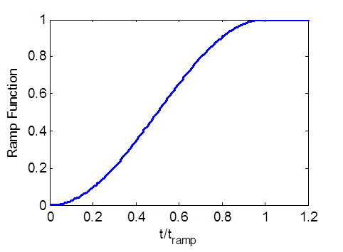
For most coastal applications, the model is initialized from a “cold start”, which means that the water level and current velocities are initially set to zero. The ramp period allows the model to slowly transition from the ini-tial condition without “shocking” the system. In CMS, the ramp function is defined as

$f_{Ramp}={\frac {1}{2}}-{\frac {1}{2}}cos\left[\pi min(t/t_{Ramp},1)\right]$(3-26)

where t is the simulation time and $t_{Ramp}$ is the ramp duration. The ramp function provides a smooth function for transitioning from the initial condition and is plotted in Figure 3.5.

Figure 3.5. Ramp function used in CMS

The ramp function is applied to the model forcing conditions, including the wave forcing $\tau _{i}^{w}$ , surface wind $\tau _{i}^{s}$ , sediment concentration capacity $C_{tk*}$ , and significant wave height $H_{s}$ , by direct multiplication of these parameters by the ramp function at each time step during the ramp period. Boundary conditions in CMS are specified without consideration of this ramp period; therefore, the boundary conditions are also slowly transitioned from the initial condition by direct multiplication of the boundary conditions by the ramp function at each time step during the ramp period.

Hydrodynamics

Momentum and Continuity

The governing equations are solved in a segregated manner in which each governing equation is linearized and solved separately in a sequential manner within an iteration loop in order to obtain a converged solution. Coupling between the velocity (momentum) and water level (continuity) is achieved with the SIMPLEC algorithm (van Doormal and Raithby 1984). The main difficulty in solving the momentum equations is that the water level is not known a priori and must be calculated as part of the solution. The solution algorithm procedure is described below. First, an initial pressure $p^{*}=\rho g{\overline {n}}^{*}$ is estimated based on the previous time step value. Then, the momentum equations are solved for the corresponding velocity

${\frac {\partial (hV_{i}^{*})}{\partial t}}+{\frac {\partial (hV_{j}^{*}V_{i}^{*})}{\partial x_{j}}}={\frac {\partial }{\partial x_{j}}}\left(v_{t}h{\frac {\partial V_{i}^{*}}{\partial x_{j}}}\right)-{\frac {h}{\rho }}{\frac {\partial p^{*}}{\partial x_{i}}}+S_{i}^{*}$(3-27)

where $S_{i}^{*}$ includes all the remaining terms. The inter-cell velocities are calculated with a Rhie and Chow (1983) type interpolation method

$V_{f}^{*}=(H_{\perp }^{*})_{f}-\left({\frac {\Delta A_{P}}{a_{P}}}\right)_{f}\left({\frac {h}{\rho }}\bigtriangledown _{\perp }p^{*}\right)_{f}$(3-28)

where $(H_{\perp }^{*})_{f}=V_{\perp }^{*}+{\frac {\Delta A_{p}}{a_{p}}}{\frac {h}{\rho }}\bigtriangledown _{\perp }p^{*}$ and $\left({\frac {h}{\rho }}\bigtriangledown _{\perp }p^{*}\right)_{f}$ denotes the linear interpolation operator. This method avoids the checkerboard oscillations associated with the collocated grid. It is noted that this approach is slightly different from Lai (2010) and others and was found to be significantly more stable.

Next, the velocity $V^{'}$ and pressure corrections $p^{'}$ are defined such that both the momentum and continuity equations are satisfied

$V_{i}^{n+1}=V_{i}^{*}+V_{i}^{'},p^{n+1}=p^{*}+p^{'}$(3-29a,b)

Subtracting the initial velocity equation from the momentum equation leads to velocity correction equation

${\frac {\partial (hV_{i}^{'})}{\partial t}}+{\frac {\partial (hV_{i}^{'}V_{j}^{'})}{\partial x_{j}}}={\frac {\partial }{\partial x_{j}}}\left(v_{t}h{\frac {\partial V_{i}^{'}}{\partial x_{j}}}\right)-{\frac {h}{\rho }}{\frac {\partial p^{'}}{\partial x_{i}}}$(3-30)

This equation can be written in the discretized form as

$a_{p}V_{i,P}^{'}=\sum a_{N}V_{i,N}^{'}-{\frac {h}{\rho }}\bigtriangledown _{i}p_{P}^{'}\Delta A_{P}$(3-31)

In the SIMPLEC algorithm, the velocity correction is assumed to vary smoothly so that $\sum a_{N}V_{i,N}^{'}$ may be approximated as $V_{i,P}^{'}\sum a_{N}$ , which leads to the velocity correction equation

$V_{i}^{'}=-G\bigtriangledown _{i}p^{'}$(3-32)

where

$G=(h\Delta A_{p}/\rho )/\left(a_{p}-\sum a_{N}\right)$ . Using $\partial h/\partial t=\partial p/(\rho g\partial t)$

and substituting $V_{i}^{n+1}=V_{i}^{*}+V_{i}^{'}$ in the continuity equation yields the semi-discrete water level correction equation

${\frac {(1+0.5\theta )(p^{*}+p^{'})-(1+\theta )p^{n}+0.5\theta p^{n-1}}{\rho g\Delta t}}={\frac {\partial }{\partial x_{j}}}\left(hG{\frac {\partial p^{'}}{\partial x_{j}}}\right)-{\frac {\partial (hV_{j}^{*})}{\partial x_{j}}}$(3-33)

Note that at convergence, $p^{'}=0$ and the Equation 3-28 reduces to the continuity equation. Once the pressure correction equation is solved, the cell-centered water levels and current velocities are corrected. The cell face velocities are also corrected as $V_{f}^{n+1}=V_{f}^{*}+V_{f}^{'}$ , in which the velocity correction is given by $V_{f}^{'}=-G_{f}(\bigtriangledown _{\perp }p^{'})_{f}$ .

Summary of the SIMPLEC Algorithm:

1. Guess the water level and pressure field $p^{*}$

2. Solve the momentum equations (give Equation numbers here) to obtain $V_{i}^{*}$

3. Use the Rhie and Chow (1983) momentum to determine the velocities and fluxes at cell faces

4. Solve the pressure equation (give Equation number here) to obtain $p^{'}$

5. Use the correction equations to adjust the velocities and water levels

6. Treat the corrected water level and pressure field as a new guess, and repeat this procedure from Step 2 until convergence

Wetting and Drying

During numerical simulations of the surface water flows with sloped beaches, sand bars, and islands, the land-water interface changes with time. This means that it is possible for nodes at the land-water interface to be wet or dry throughout a given simulation. In CMS, a threshold water depth is used to judge drying and wetting. If the depth at the cell center is larger than the threshold value (i.e. a small value such as 0.02 m for field cases), then the node is considered to be wet. Similarly, if the depth at the cell center is smaller than the threshold value, then the node is considered to be dry. For the implicit solver, all of the wet and dry cells are included in the matrix solver. Dry cells are assigned with a zero velocity. Cell faces are classified as either open (if the two cells neighboring cells are wet) or closed (i.e. cell faces are not classified as wet or dry).

Sediment Transport

Transport Equations

The sediment transport equations are discretized using the methods de-scribed in the previous section entitled General Transport Equation and are not repeated here.

Mixing Layer

The mixing layer or active layer thickness calculation is slightly modified to avoid excessively small layers and for cases of strong deposition as

$\delta _{1}=min\left[max(\delta _{1,min},2d_{50},\Delta /2),\delta _{1,max}\right]$(3-34)

where $\Delta$ is the bed form height and $\delta _{1,min}$ and $\delta _{1,max}$ are the user speci-fied the minimum and maximum mixing layer thicknesses, respectively.

'Bed Material Sorting

The bed material sorting equation (Equation 2-53) is discretized as

$\delta _{1}^{n+1}p_{1k}^{n+1}=\Delta z_{bk}+\delta _{1}^{n}p_{1k}^{n}+\Delta z_{2}p_{k}^{*n}$(3-35)

where $\Delta z_{2}=\delta _{1}^{n+1}-\delta _{1}^{n}-\Delta z_{1}$ is the change in the top elevation of the second bed layer and $p_{k}^{*n}=p_{1k}^{n}$ for $\Delta z_{2}\geq 0$ and $p_{k}^{*n}=p_{2k}^{n}$ for $\Delta z_{2}<0$ . The bed material gradation in the second layer is calculated from the following discretized form of Equation 2-54

$\delta _{2}^{n+1}p_{2k}^{n+1}=\delta _{2}^{n}p_{2k}^{n}-\Delta z_{2}p_{k}^{*n}$(3-36)

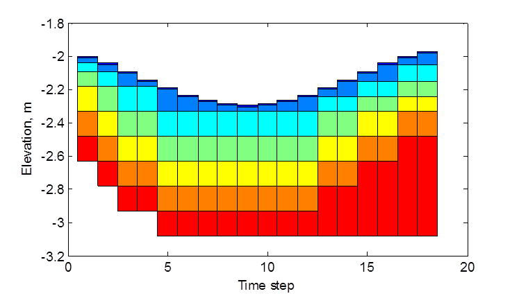
In order to avoid sediment layers from becoming extremely thin or thick, a layer merging and splitting algorithm is implemented between layers 2 and 3. Here, the subscript s corresponds to the second layer. To illustrate the bed layering process, Figure 3.6 shows an example of the temporal evolution of 7 bed layers during erosional and depositional regimes.

Figure 3.6. Example bed layer evolution. Colors indicate layer number.

Avalanching

When the slope of a non-cohesive bed,$\phi _{b}$ , is larger than the angle of repose, $\phi _{R}$ , the bed material will slide (avalanche) to form a new slope ap-proximately equal to the angle of repose. The process of avalanching is simulated by enforcing $|\phi _{b}|\leq \phi _{R}$ while maintaining mass continuity between adjacent cells. The following equation for bed change due to ava-lanching is obtained by combining the equation for angle of repose and the continuity equation between two adjacent cells:

$\Delta z_{b,p}^{a}=-\alpha _{a}\sum _{N}{\frac {\Delta A_{N}|\delta _{N}|}{\Delta A_{P}+\Delta A_{N}}}(tan\phi _{b}-sgn\phi _{b}tan\phi _{R}))H(|\phi _{b}|-\phi _{R})$(3-37)

where $\delta _{N}$ is the cell center distance between cells P and N , $\Delta$ is the cell area, $\alpha _{a}$ is an under-relaxation factor (approximately 0.25-0.5), and H(X) is the Heaviside step-function representing the activation of avalanching and equal to 1 for $X\geq 0$ and 0 for X < 0. The sign function, sgn X , is equal to 1 for $X\geq 0$ and -1 for $X<0$ and accounts for the fact that the bed slope may have a negative or positive sign. Equation 3-32 is applied by sweeping through all computational cells to calculate $\Delta z_{b}^{a}$ and then modifying the bathymetry as $z_{b}^{m+1}=z_{b}^{m}+\Delta z_{b}^{a}$ . Because avalanching between two cells may induce additional avalanching at neighboring cells, the above sweeping process is repeated until avalanching no longer occurs.

The under-relaxation factor, $\alpha _{a}$ , is used to stabilize the avalanching pro-cess and to avoid overshooting since the equation is derived considering only two adjacent cells but is summed over all (avalanching) neighboring cells. Equation 3-32 above may be applied to any grid geometry type (i.e. triangles, rectangles, etc.) and for situations in which neighboring cells are joined at corners without sharing a cell face.

Hard bottom

The sediment transport and bed change equations assume a loose bottom in which the bed material is available for entrainment. However, hard bottoms may be encountered in practical engineering applications where bed materials are non-erodible, such as bare rocks, carbonate reefs, and concrete coastal structures. Hard-bottom cells in CMS are handled by modifying the equilibrium concentration as $C_{t*}^{'}=min(C_{t*},C_{t})$ in both the sedment transport and bed change equations. The bed-slope term in the bed change equation is also modified so that only deposition (no erosion) may occur at hard-bottom cells.

Implicit Semi-Coupling Procedure

For a semi-coupled sediment transport model, the sediment calculations are decoupled from the hydrodynamics but the sediment transport, bed change, and bed material sorting equations are coupled at the timestep level and thus solved simultaneously. A modified form of the iteration procedure of Wu (2004) is implemented in CMS. The equations are ob-tained by substituting $C_{t*k}^{n+1}=p_{1k}^{n+1}C_{tk}^{n+1}$ into the bed change and sorting equations and then substituting the sorting equation into the bed change equation.

The solution procedure of sediment transport in CMS is as follows:

1. Calculate bed roughness’s and bed shear stresses

2. Estimate the potential sediment concentration capacity $C_{tk}^{*n+1}$

3. Guess the new bed composition as $p_{bk}^{n+1}=p_{bk}^{n}$

4. Calculate the fractional concentration capacity $C_{t*k}^{n+1}=p_{bk}^{n+1}C_{tk}^{*n+1}$

5. Solve transport equations for each sediment size class

6. Estimate the mixing layer thickness.

7. Calculate the total and fractional bed changes

8. Determine the bed sorting in the mixing layer

9. Update the bed elevation

10. Repeat Step 4 and iterate until convergence

11. Calculate the bed gradation in the bed layers below the mixing layer

12. Calculate avalanching

13. Correct the sediment concentration due to flow depth change $C_{tk}^{n+1}=hC_{tk}^{n+1}/h^{n+1}$

Surface Roller

The surface roller transport equation is solved in CMS-Wave using a finite difference method. The source terms are calculated at the grid cell centers. The advective or transport term is approximated using either the first-order or second-order upwind finite difference scheme. The first order upwind scheme is given by

${\frac {\partial (S_{sr}c_{j})}{\partial x}}{\bigg |}_{i,j}=\left\{{\begin{aligned}&{\frac {(S_{sr}c_{j})_{i,j}-(S_{sr}c_{j})_{i,j-1}}{\delta x_{i,j-1}}},{\text{for }}c_{i,j}>0\\&{\frac {(S_{sr}c_{j})_{i,j+1}-(S_{sr}c_{j})_{i,j}}{\delta x_{i,j}}},{\text{for }}c_{i,j}<0\end{aligned}}\right.$(3-38)

where $S_{sr}=2E_{sr}$ and i and j indicate the position along either the rows or columns, and $\delta x_{i,j}$ is the cell-center distance between adjacent cells in the j^th direction and at position i. The second-order upwind scheme is given by

${\frac {\partial (S_{sr}c_{j})}{\partial x_{j}}}{\bigg |}_{i,j}=\left\{{\begin{aligned}&{\frac {3(S_{sr}c_{j})_{i,j}-4(S_{sr}c_{j})_{i,j-1}+(S_{sr}c_{j})_{i,j-2}}{\delta x_{i,j}+\delta x_{i,j-1}}},{\text{for }}c_{i,j}>0\\&{\frac {-3(S_{sr}c_{j})_{i,j}+4(S_{sr}c_{j})_{i,j+1}-(S_{sr}c_{j})_{i,j+2}}{\delta x_{i,j}+\delta x_{i,j+1}}},{\text{for }}c_{i,j}<0\end{aligned}}\right.$(3-39)

The surface roller calculation is achieved by setting the initial roller energy and time-stepping until the steady-state solution is reached. For simplicity, an explicit Euler scheme is used as follows

$(S_{sr})^{n+1}=(S_{sr})^{n}+\Delta t_{sr}\left(-D_{r}+f_{e}D_{br}-{\frac {\partial (S_{sr}c_{j})}{\partial x}}\right)^{n}$(3-40)

where $\Delta _{sr}$ is the surface roller time step and is determined as $\Delta t_{sr}={\text{0.5 max}}(\Delta x_{j}/c){\text{ where }}\Delta x_{j}$ is the cell size in the $j^{th}$ direction. The steady-state solution is typically reached after ~40-80 time steps and takes about 1-2 seconds to run on a desktop personal computer.

Coupling Procedure of CMS-Flow and CMS-Wave

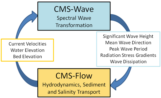
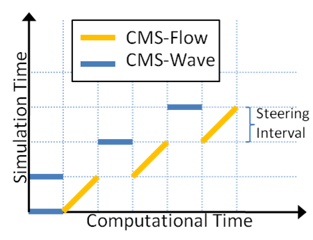
CMS-Flow and CMS-Wave can be run separately or coupled together using a process called steering (Figure 3.7). The variables passed from CMS-Wave to CMS-Flow are the significant wave height, peak wave period, wave direction, wave breaking dissipation, and radiation stress gradients. CMS-Wave uses the updated bathymetry (if sediment transport is turned on), water levels, and current velocities from CMS-Flow. The time interval at which CMS-Wave is run is called the steering interval. Currently, the steering interval is constant and the input spectra in CMS-Wave must be at constant intervals without any gaps.

Figure 3.7 CMS coupling process between CMS-Flow and CMS-Wave.

For CMS versions prior to version 4.0, the steering process is controlled in the SMS interface with communication files because the CMS-Wave and CMS-Flow models are separate executables. For CMS v4.0 and above, both CMS-Flow and CMS-Wave are contained within a single executable (known as the inline executable) and the steering process is controlled by an interval steering module. Two main advantages of the inline executable and inline steering module are: 1) the model runs faster because there is no need to use communication files or reinitialize the models (memory allocation, variable initialization, etc.) and 2) the inline executable makes the improvement and maintenance of the steering module easier for the developers and also makes the code portable for other operating systems. The inline steering process is summarized below:

1. CMS-Wave is run for the first two timesteps and the wave infor-mation is passed to CMS-Flow (Figure 3.8). If specified, the sur-face roller model is run on the wave grid and the roller contributions to the radiation stresses are added to the wave radiation stresses.

2. The wave height, period, dissipation, radiation stress gradients, and wave unit vectors are interpolated spatially from the CMS-Wave grid to the CMS-Flow grid.

3. CMS-Flow is run until the next steering interval and wave variables are linearly interpolated throughout time during the specified steering interval. At each flow timestep, variables such as wave length and bottom orbital velocities are updated using the current water depths and current velocities.

4. Water levels, current velocities, and bed elevations are estimated for the next wave timestep and are interpolated from the CMS-Flow grid to the CMS-Wave grid.

5. CMS-Wave is then run again for the following timestep.

6. Step 2-5 are repeated until the end of the simulation.

Figure 3.8. Schematic of steering process.

Spatial Interpolation and Extrapolation

CMS allows the user to use the same or different grids for CMS-Flow and CMS-Wave. If the same grid is used, then no spatial interpolation is car-ried out. If different grids are used, then spatial interpolation is necessary in order to transfer information from one model grid to another model grid. The interpolation of wave variables from the CMS-Wave grid to the CMS-Flow grid is done using a combination of bilinear and linear triangular interpolation methods. Bilinear interpolation is applied at non-jointed cells where 4 neighboring points can be identified and triangular interpolation at jointed cells. If the extents of the CMS-Wave and CMS-Flow grids are different (e.g. if the CMS-Flow grid is smaller), then the extrapolation of variables is necessary in order to avoid boundary problems with the models. Different extrapolation methods are applied to different variables and are described below.

Water levels

Water levels are extrapolated using a nearest neighbor interpolation over the entire domain, but not across land (dry) boundaries. This approach is more physically accurate than extrapolating only to a certain distance since water levels are controlled mainly by tides along the coast and the spatial variation is usually much smaller than the tidal range.

$({\bar {\eta }}_{P})_{wave}^{m}=({\bar {\eta }}_{N})_{flow}^{m}$(3-41)

where ${\bar {\eta }}_{P}$ is the water level at cell P, ${\bar {\eta }}_{N}$ is the water level at the nearest neighbor, m is the CMS-Wave timestep, and $|{\overrightarrow {r}}_{N}|$ is the distance vector from cell P to N, and $r_{x}$ is an extrapolation distance. The subscripts flow and wave indicate the CMS-Flow and CMS-Wave grids, respectively. The calculation of the water level at the CMS-Wave timestep on the flow grid is described in the section entitled Temporal Interpolation and Prediction.

Current Velocities

Current velocities are extrapolated to a certain distance referred to as the extrapolation distance. A nearest neighbor extrapolation is applied to cells within that distance and multiplied by a cosine function to produce a smooth transition from the boundary to a value of zero:

$(U_{i,P})_{wave}^{m}={\frac {1}{2}}\left\{1+cos[\pi {\text{min }}(|{\overrightarrow {r}}_{N}|/r_{x},1)]\right\}(U_{i,N})_{flow}^{m}$(3-42)

where $U_{i,P}$ is the current velocity at the extrapolated cell, $U_{i,N}$ is the current velocity at the nearest neighbor, m is the CMS-Wave timestep, and $|{\overrightarrow {r}}_{N}|$ is the distance vector from cell P to N, and $r_{x}$ is an extrapolation distance.

Bed elevations

Extrapolating bed elevations from a boundary can lead to sharp changes in bathymetry in the wave model and instability problems in both the wave and flow models. Therefore, a plausible approach is to extrapolate the bed change

$(z_{b,P})_{wave}^{m}=(z_{b,P})_{wave}^{m-1}+{\frac {1}{2}}\left\{1+cos[\pi {\text{min}}(|{\overrightarrow {r}}_{N}|/r_{x},1)]\right\}(\Delta z_{b,N})_{flow}^{m}$(3-43)

where $z_{b,P}$ is the bed elevation the extrapolated cell, $z_{b,N}$ is the bed elevation at the nearest neighbor, m is the CMS-Wave timestep, and $|{\overrightarrow {r}}_{N}|$ is the distance vector from cell P to N, and $r_{x}$ is in this case the flow grid extrapolation distance.

Significant Wave height

The significant wave height is extrapolated in the same way as the current velocities to a certain distance referred to as the extrapolation distance. A nearest neighbor extrapolation is applied to cells within that distance and multiplied by a cosine function to produce a smooth transition from the boundary to a value of zero:

$(H_{s,P})_{flow}^{n}={\frac {1}{2}}\left\{1+cos[\pi {\text{min }}(|{\overrightarrow {r}}_{N}|/r_{x},1)]\right\}(H_{s,N})_{wave}^{n}$(3-44)

where $H_{s,P}$ is the significant wave height velocity at the extrapolated cell, $H_{s,N}$ is the current velocity at the nearest neighbor, n is the CMS-Wave timestep, and $|{\overrightarrow {r}}_{N}|$ is the distance vector from cell P to N, and $r_{x}$ is in this case the wave (right?) grid extrapolation distance.

Peak Wave Period

The peak wave period is extrapolated in a similar way as the water levels using a nearest neighbor extrapolation over the entire domain, but not across land (dry) boundaries. This approach is more physically plausible than extrapolating to a finite distance and would produce zero wave peri-ods over the ocean domain (which is not physically meaningful).

Mean Wave Direction

The mean wave direction is first converted to wave unit vectors and these unit vectors are extrapolated in space. Wave unit vectors are also extrapo-lated over the entire domain, except across land (dry) boundaries, without consideration of an extrapolation distance. This approach leads to more physically plausible results.

Temporal Interpolation and Prediction

Because CMS-Wave requires the water surface elevation at times that are ahead of the hydrodynamic model, the water surface elevation and currents must be predicted for the CMS-Wave timestep. If the steering is relatively small (<30 min), then the values from the last time step may be used without significant error.

$(U_{i})_{flow}^{m}=(U_{i})_{flow}^{n}\quad ({\bar {\eta }})_{flow}^{m}=({\bar {\eta }})_{flow}^{n}\quad (z_{b})_{flow}^{m}=(z_{b})_{flow}^{n}$(3-45 a,b,c)

where m is the CMS-Wave time step, n is the last CMS-Flow time step, and the subscript flow indicates the variables on the CMS-Flow grid. For many coastal engineering applications, it is desirable and common to use relatively large steering intervals of 2-3 hours. For large steering intervals, the change in water depth has the largest influence on the nearshore wave heights. Therefore, when using large steering intervals, it is desirable to make better predictions of water levels and not use the previous timestep water levels. In cases where the relative surface gradients at any time are much smaller than the mean tidal elevation, a better approximation of water level may be obtained by decomposing the water level into

$({\bar {\eta }})_{flow}^{m}=({\bar {\eta }})_{flow}^{m}+({\bar {\eta }}_{v})_{flow}^{m}$(3-46)

where ${\bar {\eta }}_{m}$ is the mean water level and ${\bar {\eta }}_{v}$ is a variation around the mean due to due to tidal, wave, and wind generated surface gradients. ${\bar {\eta }}$ can be estimated from water level boundary conditions and is generally much larger, so ${\bar {\eta }}_{v}$ may be neglected. The surface gradient term may be approx-imated as

$({\bar {\eta }}_{v})_{flow}^{m}\approx ({\bar {\eta }}_{v})_{flow}^{n}=({\bar {\eta }})_{flow}^{n}-({\bar {\eta }}_{m})_{flow}^{n}$(3-47)

For most coastal inlet applications, Equation 3-42 is a better representation of the water surface elevation and is used as the default in CMS. After spatially interpolating the wave height, period, dissipation, and forcing onto the CMS-Flow grid, the variables are linearly interpolated in time. The wavelength, bottom orbital velocities, and mean wave-current bottom friction are then updated including current-wave interactions at each time step.

Summary