Utilities

Time Series Analysis

filter1d.m

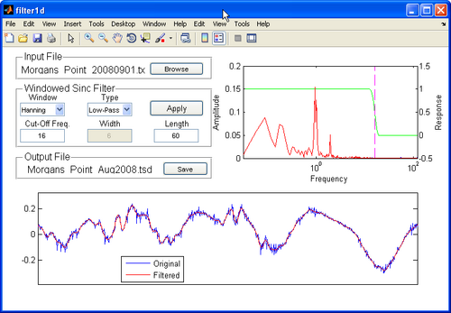
Filter1D: Time Series Analysis Tool

• The Matlab utility provides users of the SMS, a one-stop package for preparing model input time series and allows users to interpolate, resample, filter, and transform any type of model forcing and supports SMS compatible file formats for ease of data transfer.
• The main feature of the software is the ability to apply high-pass, low-pass, band-pass, and band-stop filters to time series.
• Filter1D uses a windowed sinc filter which is a non-recursive finite impulse response filter.
• Wiki Manual Filter1d
• Download Matlab script filter1d.m

TAP Interface

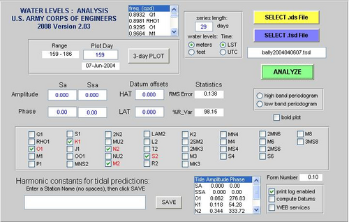
TAP: Tidal Analysis and Prediction software

• • TAPtides is the ideal package to explore and develop preliminary or finalized tidal predictions from serial records spanning several weeks to several months.
  • Designed to be easy to use, its Graphical User Interface permits quick separation of a time series of water level measurements into its tidal and non-tidal components using a selective least squares harmonic reduction employing up to 35 tidal constituents.
  • After saving the tidal constants for the constituents selected during analysis, the user can generate predictions of the astronomical tide, the water level that varies at known tidal frequencies attributable to gravitational interactions between the earth, moon, and sun.
• Wiki Manual for TAPtides TAPtides
• Wiki Manual for TAPcurrents TAPcurrents
• Download software TAP.rar

Post-processing

• Sediment transport integration tool

Matlab scripts

Read CMS-Flow solution files

• Description: Reads the CMS-Flow XMDF (*.h5) solution file in Matlab. Can read individual datasets are the whole solution.
• Usage:

filename = 'test_sol.h5';
sol = readcmsh5(filename);
wse = readcmsh5(filename,'Water_Elevation');
[wse,uv] = readcmsh5(filename,'Water_Elevation','Current_Velocity');

• Download Matlab script readcmsh5.m

Read SMS Time Series Data File

• Reads the Surface-water Modeling System time-series data (*.tsd) file in Matlab.
• Usage:

[t,dat,name,units] = read_tsd('data.tsd');

• Download Matlab script read_tsd.m.

Bin scatter data

Example of xyzbin.m application to multibeam data with 5-m bins.

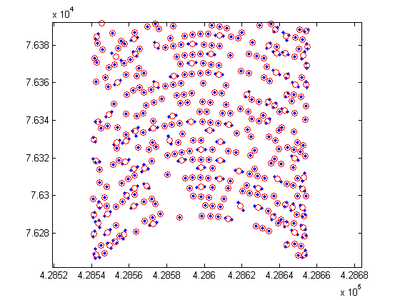
• Description: Averages the x, y, and z values of points within the same bin. The grid used to define the bins may be user specified are calculated based on the extent of the scatter points.
• Usage:

[x,y,z] = xyzbin(...);
[x,y,z] = xyzbin('infile',infile,'outfile',outfile,'dx',dx);
[x,y,z] = xyzbin('x',xin,'y',yin,'z',zin,'dx',dx);
[x,y,z] = xyzbin('x',xin,'y',yin,'z',zin,'dx',dx,'dy',dy);
[x,y,z] = xyzbin('infile',infile,'dx',dx,'x0',x0,'y0',y0,'theta',theta);

• Download Matlab script xyzbin.m.

Interpolation of CMS-Wave Spectra

• Description: Interpolates the energy spectra in the CMS-Wave *.eng file to a specified output interval which may be specified in intervals or time units (hours). For example, an output interval of 0.5 index units, interpolates the spectra at half intervals. This subroutine is useful for filling small gaps in CMS spectra.
• Usage:

interp_eng('Wave.eng','New.eng',1,0.5) %interpolates to every half interval
interp_eng('Wave.eng','New.eng',1,2)   %resamples every two spectra
interp_eng('Wave.eng','New.eng',2,1)   %hrs

• Download Matlab script interp_eng.m.

Principle Component Analysis of Vector Time Series

Example of a principle component analysis.

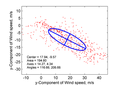
• Description: Calculates the principle axes of vector time series data. This subroutine is useful for determining the main direction of fluid flow and extracting the velocity component along the major axis. The principle axes are determined by solving the eigenvalue problem for two-dimensional scatter data.
• Usage:

s = uv2ellipse(u,v);
s = uv2ellipse(u,v,show);  %show=1 - Plots results
s = uv2ellipse(u,v,show,pos); %pos - displays a table on figure with results at pos=(x,y)

• Output:

s = Structure with the following fields:

area = Area del ellipse

axes = Magnitude of ellipse axes [major, minor];

vartotal = Total variance

Percentages = Percentage variance for each axes

Angles = Angles for each axes in degrees [major, minor];

excen = Excentricity of the ellipse

ellipse = Points [x,y] which describe the ellipse

Slope = Slope of the linear fit which goes through the origin

Center = Center of the ellipse [cu,cv]

• Note: An alternative simple way of determining the principle axes of vector time series is

$\phi _{p}={\frac {1}{2}}\arctan ^{-1}{\biggl (}{\frac {2{\big \langle }uv{\big \rangle }}{{\big \langle }v^{2}{\big \rangle }-{\big \langle }u^{2}{\big \rangle }}}{\biggr )}+{\frac {\pi }{2}}$

(1)

• Download Matlab script uv2ellipse.m:.

Spectral Analysis

Example of Power Spectrum for an idealized water level time series with white noise and a large gap.

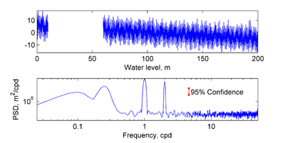
• Description: Calculates the spectrum for a scalar time series using Welch's method. The confidence intervals are calculated with the inverse of chi-square distribution. Also includes a filtering option using the butterworth filter to see the effect of the filter on the spectrum.
• Usage:

q = specwelch(x,dt,w,Nsg,pnv,Wn,ftype,n);
[psdf,f] = specwelch(x,dt,w,Nsg,pnv,Wn,ftype,n);
[psdf,conf,f] = specwelch(x,dt,w,Nsg,pnv,Wn,ftype,n);

• Input:

x - Time series, [vector]

dt - Sampling Rate, [scalar]

win - Window, one of: 'hanning', 'hamming', 'boxcar'

Nsg - Number of Segments (>=1)

pnv - Percentage Noverlap of Segments (0-100)

Nb - Band Averaging, number of bands to average

P - Probability for confidence intervals, (e.g. 0.95)

Wn - Cut-Off frequencies, used for filtering

ftype - Type of filter, 'high', 'low' or 'stop'

n - Number of coefficients to use in the Butterworth filter

• Output:

q - structure with the following fields:

xp - detrended x

f - Frequencies

T - Periods

m - Magnitude

a - Amplitude

s - Power spectrum, Sxx(win), [Power]

psdw - Power Spectrum Density, Pxx(win), [Power/rad/sample]

psdf - Power Spectrum Density, Pxx(f), [Power/sample-freq]

psdT - Power Spectrum Density, Pxx(T), [Power*time-unit]

conf - Upper and Lower Confidence Interval multiplication factors using chi-squared approach

• Download Matlab script specwelch.m:.

Vector Plot

Example comparisons between feater.m, quiver.m, and vecplot.m

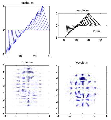
• Description: Plots directionally correct vectors. Both of matlab subroutines feather.m and quiver.m do not preserve the correct vctor angles.
• Usage:

h = vecplot(x,y,u,v,'PropertyName',PropertyValue,...)
h = vecplot(u,v,'PropertyName',PropertyValue,...)

• Input:

x,y = Position Coordinates

u,v = Vector Componentes

• Optional Properties

'DataAspectRatio' = Scaling factor between x and y axes. This is set as the second element of the property 'DataAspectRatio'

'LengthScale' = Length scaling factor for the barbs or arrows

'LineSpec' = Line specification string syntax (default '-k^') (e.g. '^k' - plots black arrows, 'k' - plots black sticks)

'Linewidth' = Linewidth

'Marker' = '^' for triangle arrows, 'v' for angled arrows,

and for stick plots (default stick)

'MarkerFaceColor' = Arrow fill color (default none)

'MarkerEdgeColor' = Arrow edge color (default line color)

'MarkerSize' = Marker size

'LegendLength' = Sets the length of the legend vector

'LegendUnits' = Sets the units for the legend vector

'legendPosition' = Sets the legend position (normalized units 0-1)

• Output:

h = handles for plot objects

• Download Matlab script vecplot.m:.

Extract Time Series from NOAA World Blended Sea Winds

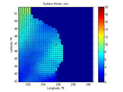
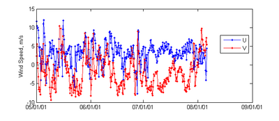
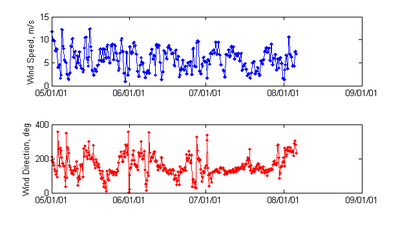
• Description: Extracts a time series of wind speed and direction for use in CMS from the 6 hrly global blended sea wind database (http://www.ncdc.noaa.gov/oa/rsad/air-sea/seawinds.html) which has a 0.25º resolution. Outputs *.xys files which can easily be imported into SMS.
• Download Matlab script blended_winds_extract_time_series.m

Blended Surface Sea Winds for a section of the North-West US coast.

Extracted sea winds

Extracted sea winds

x,y = Position Coordinates

u,v = Vector Componentes

• Output:

h = handles for plot objects

• Download Matlab script vecplot.m:.

Image Digitization Tool

• Description: digitize is a user interfase that allows to import image files (.bmp, etc) into MatLab to digitize data from. Previous sessions can also be loaded. It is useful for digitizing plots%and making world files for images.
• Instructions:

• Load image

1. To start a new session, click on the "Load" menu and select "Image File".
2. To load a saved session, click on the "Load" menu and select "Session".

• Reference the image

1. Click on the "Transformation" menu and select "Add Points".
2. Left-click on the points reference points and Right-click when finished.
3. Right-click on any reference point and select "Reference" to enter the points "true" coordinate.
4. When the coordinated for all the reference points have been entered the "Reference Data Complete" item under the "Transformation" menu will be checked.
5. To delete Transformation points, right-click on a point and select "Delete".

• Digitize Points

1. Click on the "Digitization" menu and select "Add Points". The digitized points may be entered at any time, but their transformed coordinated are not calculated until the reference data is complete.
2. To see a digitized point's transformed coordinate, right-click on a point and select "Coordinates".

• Export the Digitized Points

1. Click on "Export" and select one of the output options including variables to the workspace and an ASCII file.

• Download Matlab script digitize.m:.

HDFview

• HDFview is a free visualziation tool for browsing and editing HDF4 and HDF5 files.
• To download or download a free copy visit:

http://www.hdfgroup.org/hdf-java-html/hdfview/

Grain Size Distribution Analysis

• This Excel worksheet calculates statistics for many samples using several methods including Folk and Ward and the Method of Moments.

http://www.cedex.es/pipermail/rivers-list/attachments/20061004/56b4085f/gradistat-0001.xls

Wave Transformation

• Wave Watch III spectra
• WIS wave spectra
• CDIP Buoy wave spectra
• NDBC Buoy wave spectra

---

Documentation Portal