|
|
| (60 intermediate revisions by 4 users not shown) |
| Line 1: |
Line 1: |
| Normal 0 false false false MicrosoftInternetExplorer4
| | __NOTOC__ |
| | | <font size = "4">'''Representation of Rubble Mound Structures in the CMS'''</font><br> |
| [[Image:CHETN_Weirs_CMS_01.png|framed|none]]
| | <font color=red> '''''By Christopher Reed and Alejandro Sánchez'''''</font><br> |
| | | <font color=red> '''''Last Modified: September 17, 2010'''''</font> |
|
| |
| | |
| <font size = "4">'''Representation of Weirs in the'''</font> | |
| | |
|
| |
| | |
| <font size = "4">'''Coastal Modeling System'''</font> | |
| | |
|
| |
| | |
| '''''By Christopher Reed and Alejandro Sánchez''''' | |
| | |
|
| |
| | |
| ---- | | ---- |
| | ==Introduction== |
| | Rubble mound structures are a common coastal engineering structure used for shoreline protection and flow and sediment transport control. They are typically used as seawalls, groins, breakwaters and jetties. The design of rubble mound structures often consists of a core of small to medium size rock or riprap covered with larger rock or riprap to armor against wave energy. In coastal modeling, it is usually reasonable to assume that the flow through these structures is negligible, and they are represented as solid structures, impermeable to both flow and sediment transport. However, some rubble mounds such as that of Dana Point, CA are designed with a sufficiently large diameter core material to allow for flow and fine sediments to pass through and coarser sediment to be trapped within. |
|
| |
|
|
| | Since permeable rubble mounds are a significant control of the hydrodynamic and sediment transport in the coastal zone, it is important to include them in the CMS. An algorithm is developed based on the Forchheimer equation (1901), which represents the introduction of a non-linear term in the Darcy equation for porous media. Both the linear and non-linear coefficients in the equation are evaluated using data from studies by Gent (1995) and Sidiropoulou et al. (2007). The structures are implemented within the CMS framework by extending the steady flow equation of Forchheimer to the unsteady shallow water equations. The CMS is verified by comparing the model output to results of analytical solutions for steady flow cases. A sensitivity analysis was also conducted to determine the sensitivity of the rubble mound simulations to uncertainty in the input parameter values. |
| | |
| '''PURPOSE: '''This Coastal and Hydraulics Engineering Technical Note (CHETN) describes the representation of weirs in the Coastal Modeling System (CMS) operated through the Surface-water Modeling System (SMS). The CMS is a hydrodynamic and transport model designed for coastal and inlet applications and the SMS is a graphical user interface utility for PCs, developed by the U.S. Army Corps of Engineers (USACE). The simulation of weirs has been implemented in the CMS-Flow explicit solver. The mathematical and numerical implementation is described and examples applications are summarized.
| |
| | |
|
| |
| | |
| '''INTRODUCTION: '''Weirs are a common coastal engineering structure used to control flow and can affect sediment transport. They are typically used in weir jetties or in wetlands to control discharges, provide flood control, act as salinity barriers and optimally distribute freshwater to manage salinity regimes and sedimentation rates and deposition patterns. Since these structures are a significant component of hydrodynamic and sediment transport controls in the coastal zone, it is important that the CMS simulate their effects. The simulation of weirs is based on the standard weir equation for either sharp-crested or broad-crested weirs, with a foundation in Bernoulli<nowiki>’</nowiki>s equation. The implementation of weirs in the CMS is validated in two applications on the lower Mississippi River. The weirs are applied in the simulation of flow over the Bonne Carrie spillway north of New Orleans.
| |
| | |
|
| |
| | |
| '''COASTAL MODELING SYSTEM:''' The CMS calculates water levels, currents and waves through the coupling between a hydrodynamic model, CMS-Flow and a wave spectral model, CMS-Wave. These two models can also interact dynamically to simulate sediment and salinity transport, and morphology change (Militello, et al., 2004; Buttolph et al. 2006; Lin et al. 2008).
| |
| | |
|
| |
|
| |
|
| CMS‑Flow is a three-dimensional (3D) finite-volume model that solves the mass conservation and shallow-water momentum equations of water motion. The model can run in a two-dimensional (2-D) mode based on the depth-integrated equation. The wave radiation stress and wave field information entering the flow and sediment transport formulas in CMS‑Flow are supplied by CMS‑Wave. CMS‑Flow is forced by water surface elevation (e.g., from tide), wind and river discharge at the model boundaries, and wave radiation stress and wind field over the model computational domain. Physical processes pertinent to the present study calculated by CMS‑Flow include current, water surface elevation, sediment transport, morphology change, and representation of non-erodible bottom (e.g., structures). Additional capabilities include wetting and drying, spacially varying bottom friction, salinity transport, efficient grid storage in memory, and hot-start options.
| | == Formulation == |
| | The Forchheimer equation is conventionally written for unidirectional flow as, |
| | {{Equation|<math> I = a u + b u^2 </math>|1}} |
|
| |
|
| | where <math>I</math> is the hydraulic gradient, <math>u</math> is the bulk velocity and <math>a</math> and <math>b</math> are dimensional coefficients. The first and second terms on the right hand side represent the laminar and turbulent components of flow resistance. In order to incorporate the resistance equation in to the CMS governing equations, Fochheimer<nowiki>’</nowiki>s equation is cast into a format compatible with the steady state shallow water wave equations. In this form, the equations represents a balance between the hydraulic gradient and drag. The formulation can be extended to general applications by adding the following resistance terms to the x and y momentum equations: |
| | {{Equation|<math> |
| | R_x = -ghu(a +b\sqrt{u^2+v^2} \text{ and } R_y = -ghv(a + b\sqrt{u^2+v^2} |
| | </math>|2}} |
| | | |
| | where <math>g</math> is the acceleration due to gravity, <math>h</math> is the water depth and <math>u</math> and <math>v</math> are the bulk current velocities in the x- and y-directions. |
|
| |
|
| CMS‑Wave is a 2-D steady-state (time-independent) phase-averaged, spectral wave transformation model. The model contains theoretically derived approximations of wave diffraction, reflection, and wave-current interaction for wave simulations at coastal inlets with jetties and breakwaters. It employs a forward-marching and finite-difference method to solve the wave action conservation equation. CMS-Wave operates mainly on a coastal half-plane, so primary waves can propagate only from the seaward boundary toward shore. In the full-plane mode, CMS‑Wave performs the backward-marching for seaward spectral transformation after the forward-marching is completed.
| | The adjustable coefficients a and b in the Forchheimer equation have been evaluated in a number of studies. Three sets of formulations, proposed by Ward (1964), Kadlec and Knight (1998), and Sidiropoulou et al. (2007), are included in the CMS to determine the two coefficients. The formulas by Ward (1964) are written as |
|
| |
|
|
| | {{Equation|<math> |
| | a = \frac{360v}{gD^2} \text{ and } b = \frac{10.44}{gD}</math>|2a}} |
|
| |
|
| '''FORMULATION:''' The Hydraulic Engineering Center (HEC, 2010) approach for calculating flow over rectangular weirs is adopted here. The form of the weir flow equation as presented in HEC (2010) is:
| | The formulas of Kadlec and Knight (1998) are |
|
| |
|
|
| | {{Equation|<math> |
| | a = \frac{255v(1-n)}{gn^{3.7}D^2} \text{ and } b = \frac{2(1-n)}{gn^3 D}</math>|2b}} |
|
| |
|
| {|border="0" cellspacing="2" width="100%"
| | and the formulas of Sidiropoulou et al. (2007) read as |
|
| |
|
| | | | {{Equation|<math> |
| | a = 0.0033D^{-1.5}n^{0.08} \text{ and } b = 0.194D^{-1.285}n^{-1.14}</math>|2c}} |
|
| |
|
| |
| | In Equations (2a), (2b), and (2c), ν is the water kinematic viscosity, D is the rock or riprap diameter,and n is the porosity of rubble mound structure. |
|
| |
|
| [[Image:CHETN_Weirs_CMS_02.png|framed|none]]
| | To simulate the effects of rubble mounds, the porosity, n, is introduced in the continuity equation to account for the rubble mound void space (Reed and Sanchez 2011) |
|
| |
|
|
| | {{Equation|<math> |
| | n \frac{\partial h}{ \partial t } + \frac{\partial q_x}{ \partial x } +\frac{\partial q_y}{ \partial y } = 0 |
| | </math>|3}} |
|
| |
|
| |align = "right"|(1)
| | and similarly, in the equation of bed change due to the non-equilibrium multiple-sized transport of total-load sediment (Wu 2012) |
|
| |
|
|
| | {{Equation|<math> |
| | n (1-p'_m) \frac{\partial z_{bk}}{\partial t} = \alpha\omega_{fk}(C_k - V_{*k}) |
| | </math>|4}} |
|
| |
|
| |}
| | where <math>p^'{_m}</math> is the porosity of bed material, <math>\partial z_{bk}/\partial t</math> is the rate of the bed change due to the kth size class of sediment, <math>\alpha</math> is the total-load adaptation coefficient, <math>\omega_{fk}</math> is the sediment fall velocity, <math>C_k</math> is the depth-averaged total-load concentration of the kth size class, and <math>C_{*k}</math> is the depth-averaged |
| | total-load concentration at the equilibrium state. |
|
| |
|
|
| | == Numerical Implementation== |
| | [[File:Rubble_Figure_1.png|thumb|right|500px|Figure 1 Implementation of the Rubble Mound structure in the CMS-Flow staggered grid numerical solution scheme.]] |
|
| |
|
| where | | The implicit solver of the CMS uses a non-staggered grid |
| | for the basis of the numerical solution. The model identifies the cells where the rubble mound structures are located, as shown in Figure 2. The rubble mound resistance formulations are added to the x- and y-direction momentum equations for all the rubble mound cells. The same numerical algorithms are applied to solve the flow and sediment transport equations on the normal cells and rubble mound cells with the modifications made for rubble mound cells in Equations (3) and (4). |
|
| |
|
| [[Image:CHETN_Weirs_CMS_03.png|framed|none]]
| | The CMS-Flow model uses a staggered grid for the bases of the numerical solution. Figure 1 shows a typical grid with a set of cells marked as containing a rubble mound structure. The momentum is calculated at the cell faces. For the purpose of implementing the rubble mound representation in the numerical solution algorithm, the faces are designated as external or internal as noted in Figure 1. The rubble mound resistance formulations are added to the x- and y-direction momentum equations for all internal and external faces. In general, the same numerical approximation conventions used for evaluating variables and gradients in the standard faces and can be found in the CMS documentation (Militello et al., 2004). |
|
| |
|
| is the flow rate over the weir crest,
| |
|
| |
| [[Image:CHETN_Weirs_CMS_04.png|framed|none]]
| |
|
| |
| is the weir coefficient, L is the weir crest length, h is the upstream water level above the weir crest, and
| |
|
| |
| [[Image:CHETN_Weirs_CMS_05.png|framed|none]]
| |
|
| |
| is the submergence correction factor (also referred to as the drowned flow reduction factor). A definition schematic for both free flow and submerged flow conditions is provided in Figure 1.
| |
|
| |
|
| | In the numerical solution, the effects of wind and wave radiation stress gradients are eliminated for all rubble mound cells. There are no additional modifications to the sediment transport algorithms, other than that noted in equation 5. Bedload can be transported into a rubble mound cell. Transport within a rubble mound cell will be greatly reduced by the lower flow speed, reduced energy and subsequent lower bottom stresses. |
| | | |
|
| |
|
| [[Image:CHETN_Weirs_CMS_06.png|framed|none]]
| | The rubble mound is specified in the CMS by identifying the cells containing the rubble mound structure, and specifying the structure porosity, nominal riprap or rock diameter, and the method for specifying resistance coefficients a and b. |
|
| |
|
|
| |
|
| |
|
| Figure 1. Schematic showing weir flow conditions.
| | <br style="clear:both" /> |
|
| |
|
| | | == Resistance Coefficients a and b:== |
| | The coefficients in Fochheimer<nowiki>’</nowiki>s resistance equation have been evaluated in a number of studies. Sidiropoulou et al. (2006) provides a review of proposed formulas. The formulas by Ward (1964) are: |
| | {{Equation|<math>a = \frac{360 \upsilon}{ g D^2 } \text{ and } b = \frac{10.44}{ g D } </math>|5}} |
|
| |
|
| An inspection of Equation 1 reveals that the weir coefficient is dimensional. In CMS, the the equation is re-written as:
| | where <math>\upsilon </math> is the water dynamic viscosity and <math>D</math> is the riprap or rock diameter. Kadlec and Knight (1996) suggested the following formulas: |
| | {{Equation|<math> |
| | a = \frac{255 \upsilon (1-n) }{ g n^{3.7} D^2 } \text{ and } b = \frac{2 \upsilon (1-n)}{ g n^3 D } |
| | </math>|6}} |
|
| |
|
|
| | Sidiropoulou et al. (2006) empirically derived: |
| | {{Equation|<math> |
| | a = 0.0033 D^{-1.5} n ^{0.06} \text{ and } b = 0.194 D^{-1.26} n ^{-1.14} |
| | </math>|7}} |
|
| |
|
| {|border="0" cellspacing="2" width="100%"
| | A plot of these functions for a porosity of 0.4 and a range of diameters from 0.05 to 1.0 meters is shown in Figure 2 and 3. The largest variation in values occurs for the smaller rock size for coefficient a. The variation for parameter b is smaller, less than a factor of two over the range of rock sizes considered. |
|
| |
|
| | | | [[File:Rubble_Figure_3.png|thumb|left|500px|Figure 2. Dependence of Forchheimer<nowiki>’</nowiki>s coefficient a on rock size (porosity of 0.4).]] |
| | [[File:Rubble_Figure_4.png|thumb|none|500px|Figure 3. Dependence of Forchheimer <nowiki>’</nowiki>s coefficient b on rock size (porosity of 0.4).]] |
| | <br style="clear:both" /> |
|
| |
|
| |
| | == Additional Information== |
| | This techical wiki was prepared and funded under the Coastal Inlets Research Program (CIRP) being conducted a the U.S. Army Engineer Research and Development Center, Costal and Hydraulics Laboratory. Questions about this technical note can be addressed to to Dr. Christopher W. Reed ([mailto:Chris_Reed@URSCorp.com <font color="#0000FF"><u>Chris_Reed@URSCorp.com]</u></font>) of URS Corporation or Alejandro Sanchez ([mailto:Alejandro.Sanchez@usace.army.mil <font color="#0000FF"><u>Alejandro.Sanchez@usace.army.mil]</u></font>). The CIRP Program Manager, Dr. Julie D. Rosati ([mailto:Julie.D.Rosati@usace.army.mil <font color="#0000FF"><u>Julie.D.Rosati@usace.army.mil]</u></font>), the assistant Program Manager, Dr. Nicholas C. Kraus (Nicholas.C.Kraus[mailto:Julie.D.Rosati@usace.army.mil <font color="#0000FF"><u>@usace.army.mil]</u></font>). |
|
| |
|
| [[Image:CHETN_Weirs_CMS_07.png|framed|none]] | | Test cases showing model verification and sensitivity are provided in |
| | [[Rubble_Mound_Tests | Rubble Mound Tests]] |
|
| |
|
|
| | == References == |
| | | *Buttolph, A. M., C. W. Reed, N. C. Kraus, N. Ono, M. Larson, B. Camenen, H. Hanson, T. Wamsley, and A. K. Zundel, A. K. 2006. Two-dimensional depth-averaged circulation model CMS-M2D: Version 3.0, Report 2, sediment transport and morphology change. Coastal and Hydraulics Laboratory Technical Report ERDC/CHL-TR-06-7. Vicksburg, MS: U.S. Army Engineer Research and Development Center. |
| |align = "right"|(2)
| | *Forchheim, Ph. "Wasserbevegung durch Boden" , Z. Ver. Deutsh. Ing., Vol. 45, 1901, p.1781-1788 |
| | | *Kadlec H.R., Knight, L.R., 1996. Treatment Wetlands. Lweis Publishers. |
|
| | *Melina G. Sidiropoulou Konstadinos N. Moutsopoulos Vassilios A. Tsihrintzis (2007). Determination of Forchheimer equation coefficients a and b. Hydrological Processes, Volume 21, Issue 4, 15, Pages: 534–554. |
| | | *Militello, A., Reed, C.W., Zundel, A.K., and Kraus, N.C. 2004. Two-Dimensional Depth-Averaged Circulation Model M2D: Version 2.0, Report 1, Technical Documentation and User<nowiki>’</nowiki>s Guide, ERDC/CHL TR-04-2, U.S. Army Research and Development Center, Coastal and Hydraulics Laboratory, Vicksburg, MS. |
| |}
| | *Ward, J.C., 1964. Turbulent flow in porous media. Journal of Hydrualic Division, ASCE 90(5): 1-12 |
| | | ---- |
|
| | [[CMS-Flow:Structures | Structures]] |
| | |
| where
| |
| | |
| [[Image:CHETN_Weirs_CMS_08.png|framed|none]]
| |
| | |
| is the acceleration due to gravity and
| |
| | |
| [[Image:CHETN_Weirs_CMS_09.png|framed|none]]
| |
| | |
| QUOTE
| |
| | |
| [[Image:CHETN_Weirs_CMS_10.png|framed|none]]
| |
| | |
| . In this form, the coefficients are independent of the measurement system (i.e. Metric or English). | |
| | |
|
| |
| | |
| The value for the weir coefficient depends on the upstream and downstream geometry of the weir. Ranges for the coefficient suggested in HEC (2010) are listed in Table 1.0.
| |
| | |
|
| |
| | |
| '''Table 1.0. Suggested Weir Coefficient'''''' ''' QUOTE ''' Values.'''
| |
| | |
|
| |
| | |
| {|border="2" cellspacing="0" cellpadding="4" width="40%" align="center"
| |
| | |
| |align = "center"|'''Configuration'''
| |
| | |
| |align = "center"| QUOTE ''' Range*'''
| |
| | |
|
| |
| | |
| |-
| |
| | |
| |Sharp-crested
| |
| | |
| |align = "center"|0.55 – 0.58
| |
| | |
|
| |
| | |
| |-
| |
| | |
| |Broad-crested
| |
| | |
| |align = "center"|0.46– 0.55
| |
| | |
|
| |
| | |
| |}<br clear="all">
| |
| | |
|
| |
| | |
| <nowiki>*</nowiki> values in HEC (2010) converted to
| |
| | |
|
| |
| | |
| Super-critical flow conditions occur when the flow is independent of the tail-water elevation. These conditions occur when the tail-water elevation is sufficiently low that the sub-critical coefficient is equal to 1.0. For submerged conditions a different approach is used for setting . For sharp-crested weirs, the coefficient is based on the equation by Villemonte (1947):
| |
| | |
|
| |
| | |
| {|border="0" cellspacing="2" width="100%"
| |
| | |
| |
| |
| | |
| |
| |
| | |
| |align = "right"|(3)
| |
| | |
|
| |
| | |
| |}
| |
| | |
|
| |
| | |
| where and are defined in Figure 2. For broad-crested weirs, the value of is calculated by fitting a curve to data from USACE EM 1110-2-1603 (plate 3-5, Section A-A). An exponential curve was fit to the Section A-A data. The fit is shown in Figure 2 and the equation for C<sub>df</sub> is:
| |
| | |
|
| |
| | |
| {|border="0" cellspacing="2" width="100%"
| |
| | |
| |
| |
| | |
| |
| |
| | |
| |align = "right"|(4)
| |
| | |
|
| |
| | |
| |}
| |
| | |
|
| |
| | |
|
| |
| | |
| Figure 2. Curve fit to the USACE EM 1110-2-1603, plate 3-5, Section A-A data.
| |
| | |
|
| |
| | |
| '''NUMERICAL IMPLEMENTATION:''' The CMS-Flow explicit solver uses a staggered grid for the basis of the numerical solution. Weirs are implemented on the cell faces by specifying the two adjacent cells. The order of the cell specification is not critical for the weir implementation since the algorithm implemented in the CMS will determine the flow regime and the flow direction from the specified weir crest elevation and the water elevation in the adjacent cells. Figure 6 shows a typical CMS grid with a weir specified at a cell face.
| |
| | |
|
| |
| | |
|
| |
| | |
| Figure 6. CMS grid and designation of weirs.
| |
| | |
|
| |
| | |
| In addition to the weir location,the user must also specify the crest elevation relative to the model datum, crest length L and the coefficient QUOTE . Multiple weirs can be specified at each face and the total flow across the face is the sum of the flow calculated for each individual weir. The momentum flux associated with the flow over the weir (and subsequently across the CMS cell face) is included in both the mass balance and the momentum balance calculations. Also, a weir can be specified as ''additive'' or ''replacing'' the cell face momentum flux that is calculated using the CMS solver. When the ''replacing'' weir type is specified, the flow from all weirs associated with the cell face replaces the calculated momentum flux. If an additive weir is specified, then the final momentum flux for the cell face is calculated as the weighted sum of the weir and momentum equations fluxes:
| |
| | |
|
| |
| | |
| {|border="0" cellspacing="2" width="100%"
| |
| | |
| |
| |
| | |
| |
| |
| | |
| |align = "right"|(5)
| |
| | |
|
| |
| | |
| |}
| |
| | |
|
| |
| | |
| Where and are the momentum equations shallow water and weir equations, is the total flow across the face, and the fractions and for the momentum equation and weir flow contributions are defined as:
| |
| | |
|
| |
| | |
| : and
| |
| | |
|
| |
| | |
| The application of the ''additive'' weir type would be applicable when a weir is set in a levee or other elevated structure. In cases where the levee is over topped the flow across the levee would be a combination of the weir flow and the flow over the levee surface.
| |
| | |
|
| |
| | |
| The total flux across the cell face will be the sum of all weirs specified for that cell face. However, only the fluxes associated with the weirs will be included in the momentum balance.
| |
| | |
|
| |
| | |
| When salinity or sediment transport is included in simulations with weirs, the salinity and suspended sediment will be transported. The bedload components in sediment transport algorithms will not be transported over weirs.
| |
| | |
|
| |
| | |
| '''EXAMPLE APPLICATION:''' As an example of weir applications in the CMS, the CMS model was applied to the simulation of flow through the Bonnet Carre Spillway (BCS), which is located along the lower Mississippi River. The feasibility of locating a port facility along the Mississippi River at the Bonnet Carre Spillway was being investigated. The major concern was that the facility structures would interfere with the flow of flood waters from the Mississippi River through the spillway.
| |
| | |
| | |
| | |
| The purpose of the BCS is to divert floodwater from the Mississippi River to the Gulf of Mexico via Lake Pontchartrain. The spillway is located at River Mile 128 and was designed to pass 250,000 cfs of Mississippi River floodwater at the design stage to Lake Pontchartrain via a 5.7 mile long spillway. The BCS will be operated, in conjunction with other area structures, to divert sufficient floodwater from the Mississippi River to prevent the discharge in the Mississippi River from exceeding 1,250,000 cfs at New Orleans.
| |
| | |
|
| |
| | |
| The inlet structure of the BCS is a needle-controlled weir, located about a quarter of a mile from the riverbank. The weir is designed as a concrete gravity-over-fall dam consisting of 350 bays, each 20 feet in width, separated by 2-foot wide concrete piers. There are 176 bays in four groups, with weir crest elevations at 17.80 and 174 bays in three groups, with weir crest elevations at 15.80 ft. When in operation, the flow over the spillway weirs is free flowing, and there is no influence from the tail-water elevations.
| |
| | |
|
| |
|
| |
|
| The 2-D CMS model domain was set to extend from the upstream gage at Reserve, which is about 8 miles upstream of the BCS, down to the Carrollton gage, which is south of New Orleans and about 27 miles downstream of the BCS. The domain is shown in Figure 7 and includes an expanded view in the vicinity of the BCS. The grid spacing was set to 196.8 ft (60 m). The river levees were used to delineate the boundary since they are expected to be slightly higher than the water elevations expected in the model simulations. The grid required 16,975 cells to cover the modeling domain.
| | [[CMS#Documentation_Portal | Documentation Portal]] |
| | |
|
| |
| | |
|
| |
| | |
| Figure 7. CMS grid for BCS Weir Simulation.
| |
| | |
|
| |
| | |
| The entrance area to the BCS was included in the model as well as a short section downstream of the spillway. Since the flow over the BCS was the main concern in the analysis, and the flow of the weirs is super-critical (no tail-water effects), the downstream section is only needed to provide an outlet for the flow and the model configuration for this area does not impact the results of the analysis. The weirs were assigned along a sequence of grid cells that coincide with the physical location of the BCS.
| |
| | |
|
| |
| | |
| The grid extent was designed to coincide with gage locations so that measured data could be used as boundary conditions. Flow data from the Tarbert gage was used for the upstream flow boundary condition, and stage data from the Carrolton gage was used for the downstream water elevation boundary condition. A downstream water surface elevation for the extension of the spillway towards Lake Pontchartrain is also required, but the results of the analysis are not sensitive to the selection of this value. The value only needs to be sufficiently lower than the weir crest elevation to allow for supercritical flow over the weirs and high enough to keep the spillway submerged.
| |
| | |
|
| |
| | |
| Three scenarios were selected for the model calibration and validation. The first two are high flow cases with the BCS closed. Data from March 9, 2001 was used for the calibration case and recorded stage. Flow from January 31, 2005 was used for validation of the model. The third calibration case used data from April 22, 2008 while a major flood event occurred and for which the BCS was opened. This case was used to validate the weir function in the CMS. For all cases, the calibration consisted of comparing the predicted stage at the Reserve gage. For Case 3, a comparison of the simulated and measured flow over the BCS was assessed.
| |
| | |
|
| |
| | |
| The representation of the weirs in the model required special processing to ensure that the total length of the BCS weir system was correctly represented since the grid cells were longer than the individual BCS bays. The BCS contains 350 bays, each with a 20 ft (6.09 m) weir. Each bay is separated by a 2-foot thick wall, thus the total length of the spillway is 7,698 feet (when the last wall is not included). In order to simulate the operating conditions of the spillway bays, 40 cells were identified at the approximate location of the Bonnet Carre spillway. In order to correctly represent the total length of the BCS weirs in the model, each cell coincident with the BCS was assigned a total weir length equivalent to 8.75 bays, which is equivalent to 350 bays divided among 40 grid cells. Thus, each cell contained 175 feet of weir crest.
| |
| | |
|
| |
| | |
| Another characteristic of the BCS bays is their alternating weir crest elevations. The bays are organized into seven sections. The length of each section, number of bays and weir crest elevations are shown in Table 2. The number of cells that were used to represent each section and the corresponding weir length are provided in the last two columns. The spillway sections are numbered from west to east:
| |
| | |
|
| |
| | |
| '''Table 2. BCS Weir Configuration'''
| |
| | |
|
| |
| | |
| {|border="2" cellspacing="0" cellpadding="4" width="100%" align="center"
| |
| | |
| |align = "center"|Section (numbered from west to east)
| |
| | |
| |align = "center"|Number of Bays
| |
| | |
| |align = "center"|Elevation of Weirs (ft)
| |
| | |
| |align = "center"|Total BCS Weir Length in Section
| |
| | |
| |align = "center"|Number of Grid Cells used for Each Section
| |
| | |
| |align = "center"|Total Length (ft) of Weir Represented in Grid Cells
| |
| | |
|
| |
| | |
| |-
| |
| | |
| |align = "center"|1
| |
| | |
| |align = "center"|44
| |
| | |
| |align = "center"|17.22
| |
| | |
| |align = "center"|880
| |
| | |
| |align = "center"|5
| |
| | |
| |align = "center"|875
| |
| | |
|
| |
| | |
| |-
| |
| | |
| |align = "center"|2
| |
| | |
| |align = "center"|43
| |
| | |
| |align = "center"|15.35
| |
| | |
| |align = "center"|860
| |
| | |
| |align = "center"|5
| |
| | |
| |align = "center"|875
| |
| | |
|
| |
| | |
| |-
| |
| | |
| |align = "center"|3
| |
| | |
| |align = "center"|44
| |
| | |
| |align = "center"|17.22
| |
| | |
| |align = "center"|880
| |
| | |
| |align = "center"|5
| |
| | |
| |align = "center"|875
| |
| | |
|
| |
| | |
| |-
| |
| | |
| |align = "center"|4
| |
| | |
| |align = "center"|88
| |
| | |
| |align = "center"|15.35
| |
| | |
| |align = "center"|1,720
| |
| | |
| |align = "center"|10
| |
| | |
| |align = "center"|1,750
| |
| | |
|
| |
| | |
| |-
| |
| | |
| |align = "center"|5
| |
| | |
| |align = "center"|44
| |
| | |
| |align = "center"|17.22
| |
| | |
| |align = "center"|880
| |
| | |
| |align = "center"|5
| |
| | |
| |align = "center"|875
| |
| | |
|
| |
| | |
| |-
| |
| | |
| |align = "center"|6
| |
| | |
| |align = "center"|43
| |
| | |
| |align = "center"|15.35
| |
| | |
| |align = "center"|860
| |
| | |
| |align = "center"|5
| |
| | |
| |align = "center"|875
| |
| | |
|
| |
| | |
| |-
| |
| | |
| |align = "center"|7
| |
| | |
| |align = "center"|44
| |
| | |
| |align = "center"|17.22
| |
| | |
| |align = "center"|880
| |
| | |
| |align = "center"|5
| |
| | |
| |align = "center"|875
| |
| | |
|
| |
| | |
| |}<br clear="all">
| |
| | |
|
| |
| | |
| For Cases 1 and 2, the weir crest elevations were set to approximately 30 feet to insure that no flow passed through the spillway. The model calibration was obtained by globally adjusting the friction parameter (Manning<nowiki>’</nowiki>s n) until the model reproduced the measured upstream stage at the Reserve gage location. After a few simulations; the value of 0.019 was found to yield the best results. The velocity patterns in the vicinity of the spillway for Case 1 are shown in Figure 8. The model was then configured for the validation case (Case 2) to verify whether the model could reproduce good results for different stage and flow conditions. The results for these two cases are shown in Table 3.
| |
| | |
|
| |
| | |
| '''Table 3. Model Calibration and Validation Results.'''
| |
| | |
|
| |
| | |
| {|border="2" cellspacing="0" cellpadding="4" width="82%" align="center"
| |
| | |
| |align = "center"|'''Case ID'''
| |
| | |
| |align = "center"|'''Type'''
| |
| | |
| |align = "center"|'''Carrollton Stage (ft) (downstream boundary condition)'''
| |
| | |
| |align = "center"|'''Tarbert Flow (cfs) (Upstream flow boundary)'''
| |
| | |
| |align = "center"|'''Expected Reserve Stage (ft)'''
| |
| | |
| |align = "center"|'''Simulated Reserve Stage (ft)'''
| |
| | |
| |align = "center"|'''Percent Error'''
| |
| | |
|
| |
| | |
| |-
| |
| | |
| |1
| |
| | |
| |Calibration
| |
| | |
| |13.9
| |
| | |
| |1,097,818
| |
| | |
| |19.7
| |
| | |
| |20.2
| |
| | |
| |2.5
| |
| | |
|
| |
| | |
| |-
| |
| | |
| |2
| |
| | |
| |Validation
| |
| | |
| |15.5
| |
| | |
| |1,185,445
| |
| | |
| |22.0
| |
| | |
| |22.7
| |
| | |
| |3.2
| |
| | |
|
| |
| | |
| |-
| |
| | |
| |3
| |
| | |
| |Validation
| |
| | |
| |16.7
| |
| | |
| |1,465,000
| |
| | |
| |23.7
| |
| | |
| |23.2
| |
| | |
| |2.1
| |
| | |
|
| |
| | |
| |}<br clear="all">
| |
| | |
|
| |
| | |
|
| |
| | |
| Figure 8. CMS simulation velocity patterns for Case 1.
| |
| | |
|
| |
| | |
| The final validation was completed for Case 3, which represents the flood event of 2008, and was used to calibrate the coefficients in the CMS weir representations. The 2008 flood report (URS, 2009), which documents the 2008 flood event, provides information on which bays of the BCS were open and the total flow through each bay. The total flow was estimated to be 167,000 cfs and 160 bays were opened. The total flow through the spillway in the simulation was 169,221 cfs using a weir coefficient of 0.57 and the stage results are shown in Table 3. The simulated velocity patterns for the flow through the spillway are shown in Figure 9. The effect on the staggered open bays is evident in the flow patterns.
| |
| | |
|
| |
| | |
|
| |
| | |
| Figure 9. CMS simulation velocity patterns for Case 3.
| |
| | |
|
| |
| | |
| '''ADDITIONAL INFORMATION:''' This CHETN was prepared and funded under the Coastal Inlets Research Program (CIRP) being conducted at the U.S. Army Engineer Research and Development Center, Costal and Hydraulics Laboratory. Questions about this technical note can be addressed to to Dr. Christopher W. Reed ([mailto:Chris_Reed@URSCorp.com <font color="#0000FF"><u>Chris_Reed@URSCorp.com]</u></font>) of URS Corporation. The CIRP Program Manager, Dr. Julie D. Rosati ([mailto:Julie.D.Rosati@usace.army.mil <font color="#0000FF"><u>Julie.D.Rosati@usace.army.mil]</u></font>), the assistant Program Manager, Dr. Nicholas C. Kraus (<font color="#0000FF"><u>Nicholas.C.Kraus[mailto:Julie.D.Rosati@usace.army.mil @usace.army.mil]</u></font>). The CHETN benefited from technical reviews by Julie D. Rosati and Nicholas C. Kraus. This CHETN should be cited as follows:
| |
| | |
|
| |
| | |
| Reed, C. W., Sanchez, A. (2010) Representation of Weirs in the Coastal Modeling System. Coastal and Hydraulics Engineering Technical Note ERDC/CHL CHETN-XX-XX. Vicksburg, MS: U.S. Army Engineer Research and Development Center.
| |
| | |
|
| |
| | |
| '''REFERENCES:'''
| |
| | |
|
| |
| | |
| Buttolph, A. M., C. W. Reed, N. C. Kraus, N. Ono, M. Larson, B. Camenen, H. Hanson, T. Wamsley, and A. . Zundel, A. K. 2006. Two-dimensional depth-averaged circulation model CMS-M2D: Version 3.0, Report 2, sediment transport and morphology change. Coastal and Hydraulics Laboratory Technical Report ERDC/CHL-TR-06-7. Vicksburg, MS: U.S. Army Engineer Research and Development Center.
| |
| | |
|
| |
| | |
| Militello, A., Reed, C.W., Zundel, A.K., and Kraus, N.C. 2004. Two-Dimensional Depth-Averaged Circulation Model M2D: Version 2.0, Report 1, Technical Documentation and User<nowiki>’</nowiki>s Guide, ERDC/CHL TR-04-2, U.S. Army Research and Development Center, Coastal and Hydraulics Laboratory, Vicksburg, MS.
| |
| | |
|
| |
| | |
| URS. 2009. Hydraulic Modeling of Proposed Container Facility Along Mississippi River at Bonnet Carre<nowiki>’</nowiki> Spillway. URS Corporation, Tallahassee, FL.
| |
| | |
|
| |
| | |
| Villemonte, J.R (December 25,1947). "Submerged Weir Discharge Studies." Engineering News Record, p. 866-869.
| |
| | |
|
| |
|
| |
|
| [[category:uncategorized]] | | [[category:CMS-Flow]] |
Representation of Rubble Mound Structures in the CMS
By Christopher Reed and Alejandro Sánchez
Last Modified: September 17, 2010
Introduction
Rubble mound structures are a common coastal engineering structure used for shoreline protection and flow and sediment transport control. They are typically used as seawalls, groins, breakwaters and jetties. The design of rubble mound structures often consists of a core of small to medium size rock or riprap covered with larger rock or riprap to armor against wave energy. In coastal modeling, it is usually reasonable to assume that the flow through these structures is negligible, and they are represented as solid structures, impermeable to both flow and sediment transport. However, some rubble mounds such as that of Dana Point, CA are designed with a sufficiently large diameter core material to allow for flow and fine sediments to pass through and coarser sediment to be trapped within.
Since permeable rubble mounds are a significant control of the hydrodynamic and sediment transport in the coastal zone, it is important to include them in the CMS. An algorithm is developed based on the Forchheimer equation (1901), which represents the introduction of a non-linear term in the Darcy equation for porous media. Both the linear and non-linear coefficients in the equation are evaluated using data from studies by Gent (1995) and Sidiropoulou et al. (2007). The structures are implemented within the CMS framework by extending the steady flow equation of Forchheimer to the unsteady shallow water equations. The CMS is verified by comparing the model output to results of analytical solutions for steady flow cases. A sensitivity analysis was also conducted to determine the sensitivity of the rubble mound simulations to uncertainty in the input parameter values.
Formulation
The Forchheimer equation is conventionally written for unidirectional flow as,
|
|

|
(1)
|
where  is the hydraulic gradient,
  is the bulk velocity and
  and
and  are dimensional coefficients. The first and second terms on the right hand side represent the laminar and turbulent components of flow resistance. In order to incorporate the resistance equation in to the CMS governing equations, Fochheimer’s equation is cast into a format compatible with the steady state shallow water wave equations. In this form, the equations represents a balance between the hydraulic gradient and drag. The formulation can be extended to general applications by adding the following resistance terms to the x and y momentum equations:
|
|

|
(2)
|
where  is the acceleration due to gravity,
  is the water depth and and
  are the bulk current velocities in the x- and y-directions.
The adjustable coefficients a and b in the Forchheimer equation have been evaluated in a number of studies. Three sets of formulations, proposed by Ward (1964), Kadlec and Knight (1998), and Sidiropoulou et al. (2007), are included in the CMS to determine the two coefficients. The formulas by Ward (1964) are written as
|
|

|
(2a)
|
The formulas of Kadlec and Knight (1998) are
|
|

|
(2b)
|
and the formulas of Sidiropoulou et al. (2007) read as
|
|

|
(2c)
|
In Equations (2a), (2b), and (2c), ν is the water kinematic viscosity, D is the rock or riprap diameter,and n is the porosity of rubble mound structure.
To simulate the effects of rubble mounds, the porosity, n, is introduced in the continuity equation to account for the rubble mound void space (Reed and Sanchez 2011)
|
|

|
(3)
|
and similarly, in the equation of bed change due to the non-equilibrium multiple-sized transport of total-load sediment (Wu 2012)
|
|

|
(4)
|
where  is the porosity of bed material,
  is the rate of the bed change due to the kth size class of sediment,
  is the total-load adaptation coefficient,
  is the sediment fall velocity,
  is the depth-averaged total-load concentration of the kth size class, and
  is the depth-averaged
total-load concentration at the equilibrium state.
is the depth-averaged
total-load concentration at the equilibrium state.
Numerical Implementation
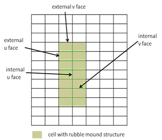
Figure 1 Implementation of the Rubble Mound structure in the CMS-Flow staggered grid numerical solution scheme.
The implicit solver of the CMS uses a non-staggered grid
for the basis of the numerical solution. The model identifies the cells where the rubble mound structures are located, as shown in Figure 2. The rubble mound resistance formulations are added to the x- and y-direction momentum equations for all the rubble mound cells. The same numerical algorithms are applied to solve the flow and sediment transport equations on the normal cells and rubble mound cells with the modifications made for rubble mound cells in Equations (3) and (4).
The CMS-Flow model uses a staggered grid for the bases of the numerical solution. Figure 1 shows a typical grid with a set of cells marked as containing a rubble mound structure. The momentum is calculated at the cell faces. For the purpose of implementing the rubble mound representation in the numerical solution algorithm, the faces are designated as external or internal as noted in Figure 1. The rubble mound resistance formulations are added to the x- and y-direction momentum equations for all internal and external faces. In general, the same numerical approximation conventions used for evaluating variables and gradients in the standard faces and can be found in the CMS documentation (Militello et al., 2004).
In the numerical solution, the effects of wind and wave radiation stress gradients are eliminated for all rubble mound cells. There are no additional modifications to the sediment transport algorithms, other than that noted in equation 5. Bedload can be transported into a rubble mound cell. Transport within a rubble mound cell will be greatly reduced by the lower flow speed, reduced energy and subsequent lower bottom stresses.
The rubble mound is specified in the CMS by identifying the cells containing the rubble mound structure, and specifying the structure porosity, nominal riprap or rock diameter, and the method for specifying resistance coefficients a and b.
Resistance Coefficients a and b:
The coefficients in Fochheimer’s resistance equation have been evaluated in a number of studies. Sidiropoulou et al. (2006) provides a review of proposed formulas. The formulas by Ward (1964) are:
|
|

|
(5)
|
where  is the water dynamic viscosity and
  is the riprap or rock diameter. Kadlec and Knight (1996) suggested the following formulas:
|
|

|
(6)
|
Sidiropoulou et al. (2006) empirically derived:
|
|

|
(7)
|
A plot of these functions for a porosity of 0.4 and a range of diameters from 0.05 to 1.0 meters is shown in Figure 2 and 3. The largest variation in values occurs for the smaller rock size for coefficient a. The variation for parameter b is smaller, less than a factor of two over the range of rock sizes considered.
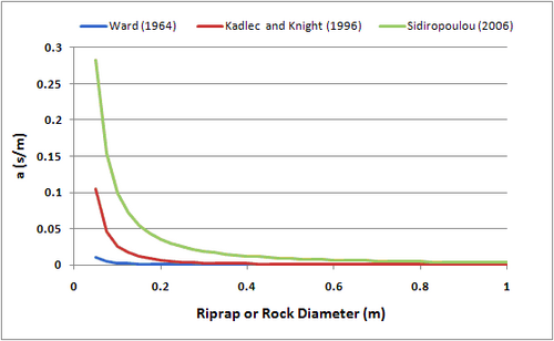
Figure 2. Dependence of Forchheimer’s coefficient a on rock size (porosity of 0.4).
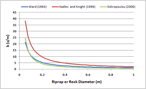
Figure 3. Dependence of Forchheimer ’s coefficient b on rock size (porosity of 0.4).
Additional Information
This techical wiki was prepared and funded under the Coastal Inlets Research Program (CIRP) being conducted a the U.S. Army Engineer Research and Development Center, Costal and Hydraulics Laboratory. Questions about this technical note can be addressed to to Dr. Christopher W. Reed (Chris_Reed@URSCorp.com) of URS Corporation or Alejandro Sanchez (Alejandro.Sanchez@usace.army.mil). The CIRP Program Manager, Dr. Julie D. Rosati (Julie.D.Rosati@usace.army.mil), the assistant Program Manager, Dr. Nicholas C. Kraus (Nicholas.C.Kraus@usace.army.mil).
Test cases showing model verification and sensitivity are provided in
Rubble Mound Tests
References
- Buttolph, A. M., C. W. Reed, N. C. Kraus, N. Ono, M. Larson, B. Camenen, H. Hanson, T. Wamsley, and A. K. Zundel, A. K. 2006. Two-dimensional depth-averaged circulation model CMS-M2D: Version 3.0, Report 2, sediment transport and morphology change. Coastal and Hydraulics Laboratory Technical Report ERDC/CHL-TR-06-7. Vicksburg, MS: U.S. Army Engineer Research and Development Center.
- Forchheim, Ph. "Wasserbevegung durch Boden" , Z. Ver. Deutsh. Ing., Vol. 45, 1901, p.1781-1788
- Kadlec H.R., Knight, L.R., 1996. Treatment Wetlands. Lweis Publishers.
- Melina G. Sidiropoulou Konstadinos N. Moutsopoulos Vassilios A. Tsihrintzis (2007). Determination of Forchheimer equation coefficients a and b. Hydrological Processes, Volume 21, Issue 4, 15, Pages: 534–554.
- Militello, A., Reed, C.W., Zundel, A.K., and Kraus, N.C. 2004. Two-Dimensional Depth-Averaged Circulation Model M2D: Version 2.0, Report 1, Technical Documentation and User’s Guide, ERDC/CHL TR-04-2, U.S. Army Research and Development Center, Coastal and Hydraulics Laboratory, Vicksburg, MS.
- Ward, J.C., 1964. Turbulent flow in porous media. Journal of Hydrualic Division, ASCE 90(5): 1-12
Structures
Documentation Portal


