The extracted water levels are stored in the CMS-Flow Model Parameters file. Below is an example of how the CMS-Flow card for the extracted wa-ter level times boundary.

Example 2-33. Extracted water level time series boundary specification using a single card.

MDRIVER_CELLSTRING "Flow_mp.h5" "PROPERTIES/Model Params/Boundary"

Step-by-Step Instructions: Extracted WSE from a Regional Model

To assign this type of BC in SMS

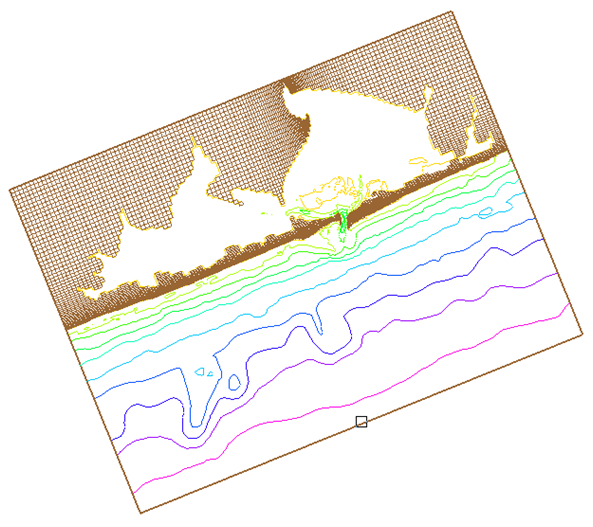
1. If not already done, load a CMS-Flow grid in SMS.

Figure 2-54. CMS-Flow grid for Shinnecock Inlet, NY.

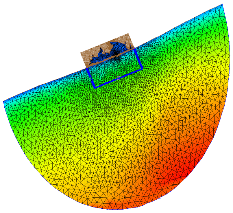
2. If not already done, load in a larger-domain (regional) simulation files including the water level solution (typically either an CMS or ADCIRC simulation).

Figure 2-55. Local CMS-Flow grid and larger-domain ADCIRC mesh for Shinnecock Inlet, NY.

3. If not already created by SMS, create the CMS-Flow cellstring at the boundary (see section Creating and Deleting Cell Strings in SMS for details).

4. Select the CMS-Flow cellstring (see section Selecting a Cellstring for details).

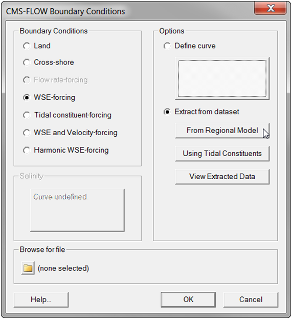
5. Open the CMS-Flow Boundary Conditions Window (see section Assigning a Boundary Condition for details). See figure below.

Figure 2-56. CMS-Flow Boundary Conditions window in SMS 11.1 with an WSE boundary condition.

6. Select WSE-forcing in the Boundary Conditions section on the left side of the window.

7. Select Extract from dataset in the Options section on the right side of the window.

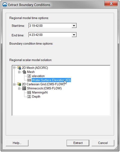
8. Click on From Regional Model. The Extract Boundary Conditions window will appear (see example figure below).

9. Select the water level forcing dataset and the start and end times for the extraction.

10. Select the Extract button in the Extract Boundary Conditions window. The window will close.

Figure 2-57. Extract Boundary Conditions window in SMS 11.1.

11. In the CMS-Flow Boundary Conditions window, select the OK button.

12. Save the SMS project File (*.sms) or CMS-Flow Simulation File (*.cmcards).

Notes:

• Due to their size, the tidal databases do come installed with SMS, and must be downloaded separately. Before using the tidal databases in SMS for the first time it is necessary to follow the steps below.

• If an ADCIRC simulation is used to extract water levels, make sure the ADCIRC grid is in the same horizontal projection as the CMS-Flow grid.

Step-by-Step Instructions: Extracted WSE using Tidal Constituents

To assign an extracted water surface elevation boundary using tidal con-stituents from a tidal database:

1. If not already done, load a CMS-Flow grid in SMS.

2. If not already created by SMS, create the CMS-Flow cellstring at the boundary (see section Creating and Deleting Cell Strings in SMS for details).

3. Select the CMS-Flow cellstring (see section Selecting a Cellstring for details).

4. Open the CMS-Flow Boundary Conditions Window (see section Assigning a Boundary Condition for details). See figure below.

Figure 2-58. CMS-Flow Boundary Conditions window in SMS 11.1 with an WSE boundary condition.

5. Select WSE-forcing in the Boundary Conditions section on the left side of the window.

6. Select Extract from dataset in the Options section on the right side of the window.

7. Click on using Tidal Constituents. The Extract Boundary Condi-tions window will appear (see example figure below).

8. Select the water level forcing dataset and the start and end times for the extraction.

9. Select the Extract button in the Extract Boundary Conditions window. The window will close.

Figure 2-59. Extract Boundary Conditions window in SMS 11.1.

10. In the CMS-Flow Boundary Conditions window, select the OK button.

11. Save the SMS project File (*.sms) or CMS-Flow Simulation File (*.cmcards).

Extracted Water Level and Velocity Time Series Boundary

The water level and velocity at a boundary can be specified as:

1. Cell-specific time-series curves (i.e. one time-series for each boundary cell). This boundary type is used when extracting boundary conditions in SMS.

2. Interpolated values from a parent grid simulation (nesting).

3. Cell-specific cosine series using interpolated tidal constituents from a tidal database.

Example 2-34. Multiple water level and velocity boundary specification using two cards.

MDRIVER_CELLSTRING "Flow_mp.h5" "PROPERTIES/Model Params/Boundary" VDRIVER_CELLSTRING "Flow_mp.h5" "PROPERTIES/Model Params/Boundary"

Cross-shore Boundary Condition

In the implicit flow solver, a cross-shore boundary condition is applied by solving the 1-D cross-shore momentum equation including wave and wind forcing (Wu et al. 2011a, 2011b). Along a cross-shore boundary, it is assumed that a well-developed longshore current exists. Thus, the along-shore (y-direction) momentum equation can be reduced to

{\frac {\partial }{\partial x}}\left(v_{t}h{\frac {\partial V_{y}}{\partial x}}\right)={\frac {1}{\rho }}(\tau _{sy}+\tau _{wy}-\tau _{by})

(2-16)

where $\tau _{sy},\tau _{wy},$ and $\tau _{by}$ are the surface, wave, and bottom stresses in the long-shore direction, respectively. The equation above is solved iteratively for the longshore current velocity. The cross-shore (x) component of the velocity is assigned a zero-gradient boundary condition.

The water level due to waves and wind at the cross-shore boundary can be determined by assuming a zero alongshore gradient of flow velocity and negligible cross-shore current velocity. For this case, the cross-shore momentum equation reduces to

\rho gh{\frac {\partial {\bar {\eta }}}{\partial x}}=\tau _{sx}+\tau _{wx}

( 2-17)

where $\tau _{sx}$ and $\tau _{wx}$ are the wind and wave stresses in the cross-shore direction.

Tidal Databases

SMS Supported Tidal Databases

SMS allows the user to generate multiple water level time series from spatially variable tidal constituents. The tidal constituents are spatially interpolated from one of several available datasets:

1. NE Pacific Tidal Database (ADCIRC)

2. NW Atlantic Tidal Database (ADCIRC)

3. LeProvost Tidal Database

Step-by-Step Instructions for Setting Up the Tidal Databases in SMS.

1. Download the tidal database. The ADCIRC database can be down-loaded from http://www.unc.edu/ims/ccats/tides/tides.htm and LeProvost from http://sms.aquaveo.com/leprovost.zip.

2. Unzip the files and save them to the SMS directory (preferably).

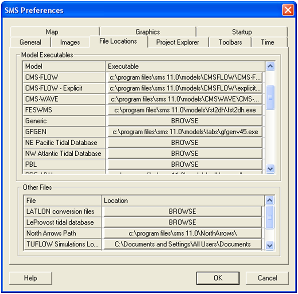
3. Set the path to the tidal database by opening SMS and clicking on the Edit menu and selecting Preferences… (see Figure 4-16).

4. Enter the correct location (path) of the tidal database.

Figure 2-60. Setting the tidal database executable location in the SMS Preferences window.

When using the SMS Boundary Extraction utility, to extract water levels or water levels and current velocities from a boundary, the SMS creates the boundary time-series are these are written to the Model Parameters File.

Advanced Boundary Specification

Boundary Blocks

In CMS versions 4.0 and earlier both the cellstring information and the boundary information were stored together in the Model Parameters File (*_mp.h5), and therefore all of the information needed for each boundary was a path within the Model Parameters File. Although simple, this method makes it difficult for users to specify their own boundary time-series without going in SMS and resaving the whole CMS-Flow project. In addition, it makes it difficult to specify additional boundary parameters. For this reason, a new approach has been adopted in CMS V4.1 which is based on block structures. Block structures offer more flexibility for specifying input parameters, make the input file more readable, and reduce the complexity of the input cards by introducing context around them. The concept of a block structure is best illustrated with the following simple example:

Example 2 35. Boundary block specification.

BOUNDARY_BEGIN

  NAME   "My Offshore Boundary" !Optional
  !Other boundary information goes here

BOUNDARY_END

In the above example is incomplete since only a name is provided for boundary and no other boundary information is given such as the forcing conditions or the location of the boundary. These are covered in the fol-lowing sections with detailed examples. A description of the boundary structure cards are provided in the table below.

Table 2-48. CMS-Flow cards related to the flux boundary condition.

Input	Format	Notes
Begins a Boundary Block	[begin=BOUNDARY_BEGIN, name=BNDblock]	Begins the block structure for a boundary condition
Boundary Block Name	[card=NAME, parent=BNDblock, optional=true] [name=bndName, type=char]	Specifies a boundary name. Optional.
Ends a Boundary Block	[end=BOUNDARY_BEGIN]	Begins the block structure for a boundary condition

Cellstrings

In CMS-Flow the spatial location of boundaries conditions is specified using cellstrings which are a list of cell ID’s corresponding to the boundary cells in the CMS-Flow grid. Once cellstrings have been created, boundary conditions can be assigned to the cellstring. Cellstrings without assigned boundary conditions or boundaries without cellstrings are assumed to be closed.

Table 2-49. CMS-Flow card for specifying cellstrings.

Input	Format	Notes
Boundary Cellstrings	[card=CELLSTRING, parent=BNDblock] [arg=bidFile, type=char, default=mpFile] [arg=bidPathID, type=char, default=none]	Specifies the boundary file, and path/ID. The path is used for XMDF files and ID number for ASCII Boundary ID Files.

Example 2-36. A boundary block structure with the cellstring boundary information specified in the Model Parameters File (*_mp.h5).

BOUNDARY_BEGIN

  CELLSTRING   "Flow_mp.h5" "PROPERTIES/Model Params/Boundary_#1"

BOUNDARY_END

Example 2-37. A boundary block structure with the cellstring boundary information specified in an ASCII Boundary ID File (*.bid).

BOUNDARY_BEGIN

  NAME        "My Offshore Boundary" !Optional
  CELLSTRING   "Boundaries.bid"  1 ![file name] [cellstring ID]

BOUNDARY_END

The Boundary ID File (*.bid) is an ASCII file with all of the cell ID’s listed for each boundary. This option allows users an alternate option to specifying boundaries which may be easier than editing the Model Parameters File. A simple example of a Boundary ID File is provided below.

Example 2-38. Boundary ID File.

2 !Number of strings 3 !Number cells in string 1 6 12 18 4 !Number of cells string 2 1 2 3 4

The lines with the number of cellstrings and the length of each cellstring must be on a separate line. However, the actual cellstring ID numbers may be on a single or multiple lines.

Notes:

• When working with advanced CMS-Flow features such as the boundary blocks, it is recommended to save a backup of the CMS-Flow Model Control File in case SMS removes or changes any cards specified in a text editor. When using many advanced cards, it is recommended to work in a text editor instead of SMS.

• Always check the CMS-Flow Diagnostic File (see Section Diagnostic File) and output screen to make sure that the input parameters and options are being set properly in the model.

Flux Boundary

Several advanced features for the flux boundary are available through the advanced cards. These features use a block structure format which allows greater flexibility in assigning boundary options. The flux boundary block and some of the basic boundary options are described in the table below.

Table 2-50. CMS-Flow cards related to the flux boundary condition

Input	Format	Notes
Flux Boundary Block	[begin=FLUX_BEGIN, name=Qblock]	Begins the block structure for a flux boundary condition
Flux data units	[card=(UNITS,FLUX_UNITS), parent=Qblock] [arg =Qunits, type=char, options=fluxunits, default=’m^3/s/cell’]	Specifies the units of the input flux data.
Inflow direction	[card=(DIRECTION, INFLOW_DIRECTION), parent=Qblock] [arg=QDir, type=float, optional=true, default=auto options=(-360<Qdir<=360 ’deg’)] [arg=QDirUnits, type=char, options=AngUnits, default=’deg’]	Specifies in the inflow angle clockwise from North. The default value is inwards normal to the boundary.
Conveyance coefficient	[card=(CONVEYANCE, CONVEYANCE_COEFFICIENT), parent=Qblock] [arg=Qconvey, type=real, range=(0.3<Qconvey<0.8), default=0.667]	Specifies the conveyance coefficient used to distribute the total flux along the boundary.
Flux Boundary Block	[end=FLUX_END, block=Qblock]	Ends the block structure for a flux boundary condition

The boundary flux may be specified as a flux per boundary cell or as a total flux for the whole boundary. The flux along the boundary and is distributed using a conveyance approach. If the flux is specified per cell, then it is multiplied by the number of cells to compute a total flux and then distributed along the boundary using the conveyance approach. The inflow direction is assumed to be normal to the boundary if not specified. The boundary flux may be specified as a constant or time-series.

Notes:

• The inflow direction is only uses for inflow conditions, as the name indicates. If the flow is outward, the flow is allowed to exit the domain without modifying the flow direction.

Flux Value

For many cases, it is sufficient to specify a constant flux. The flux value is specified using the card described in the table below.

Table 2-51. CMS-Flow cards related to the flux boundary condition.

Input	Format	Notes
Flux value	[card=(VALUE,FLUX_VALUE)] [arg=Qvalue, type=float, optional=true] [units=QvalueUnits, type=char, options=fluxunits, default=’m^3/s/cell’]	Specifies the boundary flux value.

Below is an example in which a constant total flux is applied to a bound-ary. The units of the flux value are optional. The default units are m³/s/cell.

Example 2-39. Constant boundary flux.

BOUNDARY_BEGIN

  CELLSTRING   "Flow_mp.h5" "PROPERTIES/Model Params/Boundary"
  FLUX_BEGIN
     VALUE       50.0 ‘m^3/s’ !Constant water flux
  FLUX_END

BOUNDARY_END

Flux Time Series

The boundary flux may be specified using a time-series.

Table 2-52. CMS-Flow cards related to the flux boundary condition.

Input	Format	Notes
Flux time series file	[card=(CURVE,FLUX_CURVE), parent=Qblock] [arg=Qfile, type=char, default=none] [arg=Qfath, type=char, default=none]	Specifies the Flux Data File Name (including path if different from Card File) and Dataset Path (for XMDF files only). Optional. Assumed to be the same as the cellstring if not specified.

The simple example below is equivalent to using the card QDRIVER_CELLSTRING. It uses the flux curve specified in the Model Parameters File.

Example 2-40. Total flux time-series boundary.

BOUNDARY_BEGIN

  CELLSTRING   "Flow_mp.h5" "PROPERTIES/Model Params/Boundary"
  FLUX_BEGIN
     CURVE     "Flow_mp.h5" "PROPERTIES/Model Params/Boundary" !Optional
  FLUX_END

BOUNDARY_END

The example below illustrates the enhanced capabilities of the block structure format. In the example, a name is assigned to the boundary. The cellstring ID’s are specified using a Boundary ID File (*.bid). The input total flux time series is specified in an XY Series file (*.xys). The units of the time series flux is specified as cubic meters per second. The inflow direction is assigned clockwise from true North. The conveyance coefficient determines how the total flux is distributed along the boundary. For the simple case provided below the water depths and Manning’s coefficient are constant along the boundary, so the conveyance coefficient will not affect the results.

Example 2-41. Total flux time-series specification using an XY Series file (*.xys).

BOUNDARY_BEGIN

 NAME             "River"
 CELLSTRING       "Boundaries.bid"  1 ![file name] [cellstring ID]
 FLUX_BEGIN
   CURVE          "Flux.xys"  !Contains flux data
   UNITS          ’m^3/s’     !Optional, default is m^3/s/cell
   DIRECTION      110.0 ’deg’ !Optional, -360<real<360 in degrees
   CONVEYANCE     0.5         !Optional, 0.5<real<1.0, default=0.667
 FLUX_END

BOUNDARY_END

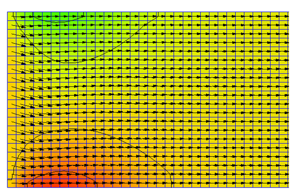
The figure below shows an example of the inflow direction specified at 110 degrees.

Figure 2-61. Example of a flux boundary specified at an oblique angle to the boundary. Contours indicate the current magnitude with warmer colors being larger current velocities.

It is also possible to use a Time Series Data or TSD file (*.tsd). The TSD file has the advantage that it uses a reference time so the input files is independent of the simulation starting time.

Example 2-42. Volume flux per cell time-series specification using a Time Series Data file (*.tsd).

BOUNDARY_BEGIN

 CELLSTRING       "Boundaries.bid"  1  ![file name] [cellstring ID]
 FLUX_BEGIN
   CURVE          "Flux.tsd"    !Contains flux data
   UNITS          ’m^3/s/cell’  !Optional, default is m^3/s/cell
   DIRECTION      90.0 ’deg’    !Normal to boundary default is 90
 FLUX_END

BOUNDARY_END

Water Level Boundary

Several advanced features for the water boundary are available through the advanced cards using the water level block structure format. The hierarchal block structures allow more flexibility in assigning input parameters, make the input file more readable and reduce the complexity of the input cards by introducing context around them. The syntax for the water level block structure is described in the table below.

Table 2-53. CMS-Flow cards related to the wse boundary condition block.

Input	Format	Notes
Begins a WSE Boundary Block	[block=WSE_BEGIN, name=WSEblock]	Begins the block structure for a flux boundary condition
Ends WSE Boundary Block	[block=WSE_END, name=WSEblock]	Ends the block structure for a flux boundary condition

The cards or input parameters which can be placed within the water level block depend on the boundary condition specification and is discussed in detail in the sections below. The boundary water levels may be specified as:

1. Single water level value

2. Multiple water level time series (one for each boundary cell)

3. Extracted water level time series from a parent simulation (nesting)

4. Tidal constituents (constant along boundary)

5. Harmonic constituents (constant along boundary)

6. Extracted water level constituents from a tidal database

The above options are described in detail in the following sections.

Single Water Level Value

The simplest water level boundary condition is a constant value. This water level boundary condition is useful for simulating steady-state problems. The input cards used for specifying a constant water level and boundary options are described in the table below.

Table 2-54. CMS-Flow cards related to the single water level time series boundary condition.

Input	Format	Notes
WSE value	[card=VALUE, parent=WSEblock] [name=WSEval, type=float, optional=true, default=0.0)]	Specifies constant WSE.
WSE gradients	[card=(WSE_GRADIENTS,GRADIENTS), parent=WSEblock] [name=WSEgrad, type=float, optional=true, default=’0.0,0.0’)]	Specifies WSE gradients which are superimposed on the boundary. Used to approximate regional circulation.
WSE correction or adjustment	[card=(ADJUSTMENT,CORRECTION), parent=WSEblock] [name=WSEadjust, type=char,options=(ON,OFF), default=ON]	Corrects the boundary water level for wind, atmospheric pressure, and wave forcing.

The following simple example illustrates how to specify a constant water level using the advanced block structure:

Example 2-43. Constant WSE BC specification using a block structure.

BOUNDARY_BEGIN

  CELLSTRING   "Boundaries.bid"  1 ![file name] [cellstring ID]
  WSE_BEGIN
     VALUE       0.2 m   !constant water level, units optional
  WSE_END

BOUNDARY_END

User Guide 007

Contents

Step-by-Step Instructions: Extracted WSE from a Regional Model

Notes:

Step-by-Step Instructions: Extracted WSE using Tidal Constituents

Extracted Water Level and Velocity Time Series Boundary

Cross-shore Boundary Condition

Tidal Databases

Step-by-Step Instructions for Setting Up the Tidal Databases in SMS.

Advanced Boundary Specification

Boundary Blocks

Cellstrings

Notes:

Flux Boundary

Notes:

Flux Value

Flux Time Series

Water Level Boundary

Single Water Level Value

Navigation menu

User Guide 007

Step-by-Step Instructions: Extracted WSE from a Regional Model

Notes:

Step-by-Step Instructions: Extracted WSE using Tidal Constituents

Extracted Water Level and Velocity Time Series Boundary

Cross-shore Boundary Condition

Tidal Databases

Step-by-Step Instructions for Setting Up the Tidal Databases in SMS.

Advanced Boundary Specification

Boundary Blocks

Cellstrings

Notes:

Flux Boundary

Notes:

Flux Value

Flux Time Series

Water Level Boundary

Single Water Level Value

Navigation menu

Search