User Guide 009
Extracted Water Level Tidal Constituents from a Database
CMS supports extracting water level tidal constituent information directly from regional and world tidal databases. The constituent information is then used internally to generate boundary information along cellstrings according to
| (2-20) |
where
- i = subscript indicating a tidal constituent
- = external boundary water surface elevation
- = mean amplitude [m]
- fi = node (nodal) factor [-]
- = frequency [deg/hr]
- t = elapsed time from midnight of the starting year [hrs]
- = equilibrium phase [deg]
- = phase lag or epoch [deg]
The nodal factor is a time-varying correction to the mean amplitude. The equilibrium phase has a uniform component and a relatively smaller periodic component. The zero-superscript of indicates that the constituent phase is at time zero.
All tidal databases have constituent information for water levels and some also have constituent information for current velocities. The table below lists the tidal databases currently supported in SMS and some basic information.
Table 2-60. Tidal Databases supported by CMS-Flow.
| Name | Description | Coverage and Grid | Water Level
Constituents |
Current
Velocity Constituents |
|---|---|---|---|---|
| EC2001 | US East Coast Tidal Database calculated with the Finite Element model ADCIRC (Mukai et al. 2002). | Western North Atlantic, Gulf of Mexico and Caribbean Sea. Unstructured triangular mesh with 254565 nodes and variable resolution ~1 – 25 km | STEADY,
K1,01,Q1, M2,S2,N2, K2,M4,M6 |
STEADY,
K1,01,Q1, M2,S2,N2, K2,M4,M6 |
| ENPAC2003 | US West Coast Tidal Database calculated with the Finite Element model ADCIRC (Spargo et al. 2004). | Eastern Pacific Ocean from Alaska to Central Mexico Coast. Unstructured triangular mesh with 272913 nodes and variable resolution of ~5 – 70 km | STEADY,
K1,01,P1, Q1,M2,S2, N2,K2,M4, M6 |
STEADY,
K1,01,P1, Q1,M2,S2, N2,K2,M4, M6 |
| LEPROVOST | Finite Element Solution based global tidal database | Interpolated rectangular grid from an unstructured triangular mesh. Grid resolution 1/2 x 1/2 deg | S2,Q1,O1,
N2,M2,MU2, K2,L2,T2, K1,2N2 |
|
| FES952 | Finite Element Solution based global tidal database based purely on hydrodynamic data (Le Provost et al. 1994) | Interpolated rectangular grid from an unstructured triangular mesh. Grid resolution 1/2 x 1/2 deg | M2,S2,N2,
K2,2N2,K1, Q1,O1,P1 |
|
| FES2004 | Finite Element Solution based global tidal database. Includes assimilation of mareographic and satellite data (Lyard et al. 2006). | Interpolated rectangular grid from an unstructured triangular mesh. Grid resolution 1/8 x 1/8 deg | M2,S2,N2,
K2,2N2,K1, Q1,O1,P1 |
The Le Provost tidal database can be downloaded from http://sms.aquaveo.com/leprovost.zip. The ADCIRC tidal databases can be downloaded from http://www.unc.edu/ims/ccats/tides/tides.htm. The FES2004 tidal database can be downloaded from http://www.legos.obs-mip.fr/en/share/soa/cgi/getarc/v0.0/index.pl.cgi?contexte=SOA&donnees=maree&produit=modele_fes.
Notes:
- • The accuracies of the nonlinearly generated constituents STEADY, M4, and M6 in the ADCIRC tidal databases have not been verified and should therefore be used with caution.
The CMS-Flow cards used to specify the tidal database information are described in the table below.
Table 2-61. CMS-Flow cards related to the tidal database boundary block.
| Input | Format | Notes |
|---|---|---|
| Begins a Tidal
Database Boundary Block |
[begin=TIDAL_DATABASE_BEGIN,
name=TCblock] |
Begins a tidal database block. |
| Tidal Database
Name |
[card=(DATABASE_NAME,NAME),
parent=TDBblock] [name=TDBname, type=char, default=none] |
Specifies the name of the tidal database. |
| Tidal Database
Path |
[card=(DATABASE_PATH,PATH),
parent=TDBblock] [name=TDBname, type=char, default=none] |
Ends the block structure for a flux boundary condition |
| Ends a Tidal
Database Boundary Block |
[begin=TIDAL_DATABASE_END,
name=TCblock] |
Ends a tidal database block. |
The example below only 4 tidal constituents are selected from the tidal database. In addition an WSE offset is specified to correct for a tidal datum shift.
Example 2-57. Tidal database water level boundary specification
BOUNDARY_BEGIN
  NAME           "Tidal Database Boundary"
  CELLSTRING     "Flow_mp.h5" "PROPERTIES/Model Params/Boundary"
  WSE_BEGIN
     OFFSET      0.1 m   !Optional, default = 0.0 m, default units = m
  WSE_END
  TIDAL_DATABASE_BEGIN
     NAME        EC2001 !EC001 | ENPAC2003 | FES95 | FES2004 | LEPROVOST
     PATH        "E:\Tidal_Databases\ec2001\"
     CONSTITUENTS 4 M2 S2 K1 O1   ![num] [cname(1:num)], optional
  TIDAL_DATABASE_END
BOUNDARY_END
Example: CMS simulation of Southern California using Tidal Databases
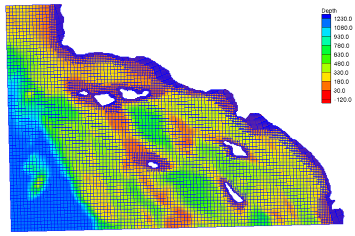
The CMS model is setup for southern California coast. The computation grid is presented in the figure below.
Figure 2-66. Example computational grid for southern California.
The offshore boundary is specified a tidal database boundary condition. The tidal dabase selected is the EC2001 database which is based on a regional ADCIRC simulation. In the case, the same regional database was used to generate the bathymetry for the CMS simulation. The CMS-Flow input cards used to specify the offshore boundary are described in the example below.
Example 2-58. Tidal database water level boundary specification.
BOUNDARY_BEGIN
  NAME           "Tidal Database Boundary"
  CELLSTRING     "Flow_mp.h5" "PROPERTIES/Model Params/Boundary"
  WSE_BEGIN
  WSE_END
  TIDAL_DATABASE_BEGIN
     NAME  ENPAC2003 !EC001 | ENPAC2003 | FES95 | FES2004 | LEPROVOST
     PATH  "E:\Tidal_Databases\ec2001\"
  TIDAL_DATABASE_END
BOUNDARY_END
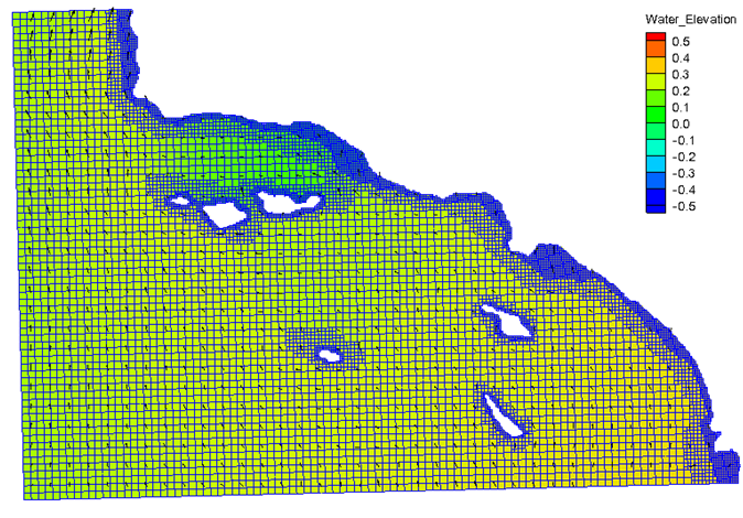
Figure 2-67. Sample water levels and current velocites for southern California forced with the water surface elevation constituents extracted from the ENPAC2003 tidal datbase.
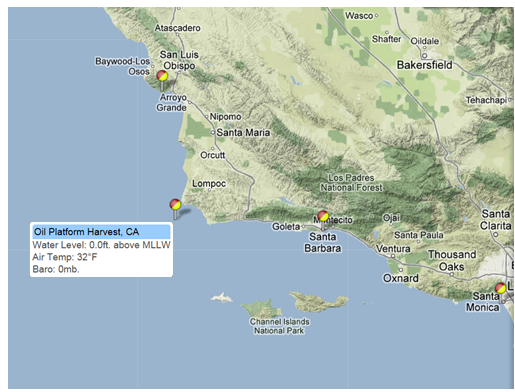
Figure 2-68. Location of Oil Platform Harvest, CA.
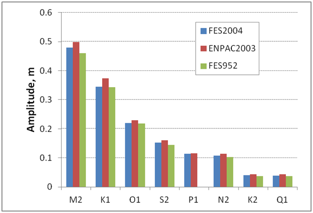
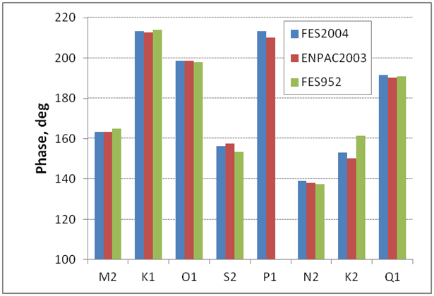
In order to show the variability in tidal constituents between different databases, the amplitudes and phases of three databases are presented in Figure 2 69 at the Oil Platform Harvest, CA. The ENPAC2003 database has the largest tidal amplitudes compared to the FES2004 and FES95.2 databases. It is noted that the FES95.2 database does not contain the P1 constituent. The phases are relatively similar with the largest differences occurring for the K2 constituent.
a.
b.
Figure 2-69. Comparison of tidal constituent amplitudes (a) and phases (b) at Oil Platform Harvest, CA, for three different tidal databases.
Mixed Water Level and Current Velocity Boundaries
There are three types of mixed water level and velocity boundary condi-tions supported using block structures
- 7. Multiple water level and velocity boundary condition
- 8. Nested water level and velocity boundary condition
- 9. Extracted water level and velocity using a tidal constituent database
Table 2-62. CMS-Flow cards related to the WSE and Currently Velocity boundary blocks.
| Input | Format | Notes |
|---|---|---|
| Begins a WSE
Boundary Block |
[block=WSE_BEGIN,
name=WSEblock] |
Begins the block structure for a flux boundary condition |
| Ends a WSE
Boundary Block |
[block=WSE_END,
name=WSEblock] |
Ends the block structure for a flux boundary condition |
| Begins a Velocity
Boundary Block |
[block=VEL_BEGIN,
name=WSEblock] |
Begins the block structure for a flux boundary condition |
| Ends a Velocity
Boundary Block |
[block=VEL_END,
name=WSEblock] |
Ends the block structure for a flux boundary condition |
Multiple Water Level and Current Velocity Time Series Boundary
TBC
Example: SMS-generated Multiple Water Levels and Current Velocities
In the example below the SMS interface is used to create a multiple water level and current velocity time-series boundary and the CMS project files are saved. The CMS-Flow card file is then modified by commenting out the SMS generated cards MULTI_HDRIVER_CELLSTRING and MULTI_VDRIVER_CELLSTRING, and placing the card information in the user-specified boundary block. It is noted that both the cellstring infor-mation and the extracted water levels are contained within the same path of the CMS-Flow Model Parameters File (*_mp.h5). This is the reason why both the CELLSTRING and DATASET cards contain the same file name and path.
Example 2-59. Multiple water level and current velocity time-series boundary specification using a block structure.
- MULTI_HDRIVER_CELLSTRING "Flow_mp.h5" "PROPERTIES/Model Params/Boundary"
- MULTI_VDRIVER_CELLSTRING "Flow_mp.h5" "PROPERTIES/Model Params/Boundary"
BOUNDARY_BEGIN
  CELLSTRING   "Flow_mp.h5" "PROPERTIES/Model Params/Boundary"
  WSE_BEGIN
     DATASET   "Flow_mp.h5" "PROPERTIES/Model Params/Boundary" !Optional
     OFFSET    0.1 m   !Optional
     TIME_INTERP_ORDER   2 !Temporal interpolation
     TIME_SMOOTH_ITER    1  !Temporal smoothing iterations
     TIME_SMOOTH_WIDTH   3 !Temporal smoothing window width
     SPACE_SMOOTH_ITER   2 !Spatial smoothing iterations
     SPACE_SMOOTH_WIDTH  3 !Spatial smoothing window width
  WSE_END
  VEL_BEGIN
     DATASET   "Flow_mp.h5" "PROPERTIES/Model Params/Boundary" !Optional
     TIME_INTERP_ORDER   1 !Temporal interpolation
     TIME_SMOOTH_ITER    1  !Temporal smoothing iterations
     TIME_SMOOTH_WIDTH   3 !Temporal smoothing window width
     SPACE_SMOOTH_ITER   2 !Spatial smoothing iterations
     SPACE_SMOOTH_WIDTH  3 !Spatial smoothing window width
  VEL_END
BOUNDARY_END
Example: User-specified Multiple Water Levels and Current Velocities TBC
Example 2-60. Excerpt of a Time Series Data file (*.tsd) used to specify water levels for a multiple water level and current velocity boundary condition.
TIME_SERIES "Boundary WSE" "Unassigned" 7 100 "01/01/2011 00:00:00"
     0.000     0.0000    0.0000    0.0000    0.0000    0.0000    0.0000
  1800.000     0.0020    0.0021    0.0022    0.0023    0.0024    0.0025
  3600.000     0.0073    0.0074    0.0075    0.0076    0.0077    0.0078
  5400.000     0.0842    0.0843    0.0844    0.0845    0.0846    0.0847
  7200.000     0.1731    0.1732    0.1733    0.1734    0.1735    0.1736
  9000.000     0.2546    0.2547    0.2548    0.2549    0.2550    0.2551
  ...
Example 2-61. Excerpt of a Time Series Data file (*.tsd) used to specify current velocities for a multiple water level and current velocity boundary condition
TIME_SERIES "Boundary Vel" "Unassigned" 13 100 "01/01/2001 00:00:00"
       0.000      0.0000     0.0000     0.0000     0.0000    …
    1800.000     -0.0022     0.0005    -0.0022     0.0005    …
    3600.000      0.0038     0.0019     0.0038     0.0019    …
    5400.000      0.0132     0.0015     0.0132     0.0015    …
    7200.000      0.0242     0.0014     0.0242     0.0014    …
    9000.000      0.0354     0.0010     0.0354     0.0010    …
   10800.000      0.0461     0.0003     0.0461     0.0003    …
   12600.000      0.0554    -0.0004     0.0555    -0.0004    …
…
Notes:
- • If the number of time steps is set to zero (forth entry in second line of TSD file), CMS will automatically determine the number from the in-put file. Therefore, the parameter may be considered optional when using as an input for CMS.
Extracted Water Levels and Current Velocities from a Parent Simulation
As described previously, CMS supports automated one-way nesting within parent CMS and ADCIRC models. When using this feature, the CMS automatically extracts the boundary condition information from the parent model solution. The user only has to specify to point to the boundary cellstring and the location and name of the parent model simulation. The user may force the CMS with either water levels or water levels and velocities extracted from the parent simulation.
The table below describes the CMS cards used to specify a nested water level boundary condition in CMS.
Table 2-63. CMS-Flow cards related to the single tidal current velocity boundary condition.
| Input | Format | Notes |
|---|---|---|
| Current Velocity solution | [card=VEL_SOLUTION,
parent=VELblock] [arg=VELsol, type=char, options=PARENT] |
Specifies the boundary as a nested current velocity boundary. |
| Current Velocity Temporal Interpolation Order | [card=TIME_INTERP_ORDER]
[arg=VELnti, type=int, range=(1<VELnti<3), default=2] |
Order of Lagrangian polynomial used to interpolate time-series. |
| Current Velocity Temporal Smoothing Iterations | [card=TIME_SMOOTH_ITER]
[arg=VELnsi, type=int, range=(0<VELnsi<10), default=2] |
Temporal smoothing iterations. Smoothing is done by a simple moving average. |
| Current Velocity Temporal Smoothing Window Width | [card=TIME_SMOOTH_WIDTH]
[arg=VELnsw, type=int, range=(0<VELnsw<10), default=0] |Temporal smoothing window width. Should be an odd number Smoothing is done by a simple moving average. |
Example: Nesting a CMS simulation within an ADCIRC simulation
If the ADCIRC simulation is 3D, it is important to export the depth-averaged current velocity file (fort.63 or *_.h5) so that this file can be used for current velocity extraction.
Example 2-62. Extracting water levels and velocities from parent ADCIRC simulation.
BOUNDARY_BEGIN
 NAME           "Nested ADCIRC wse and velocity boundary"
 CELLSTRING      "Flow_mp.h5" "PROPERTIES/Model Params/Boundary"
 WSE_BEGIN
   WSE_OFFSET   0.1 m
   TIME_INTERP_ORDER   2     !optional, temporal interpolation
   SPACE_SMOOTH_ITER   1     !optional, spatial smoothing iterations
   SPACE_SMOOTH_WIDTH  3     !optional, spatial smoothing window width
 WSE_END
 VEL_BEGIN
   TIME_INTERP_ORDER   2     !optional, temporal interpolation
   SPACE_SMOOTH_ITER   1     !optional, spatial smoothing iterations
   SPACE_SMOOTH_WIDTH  3     !optional, spatial smoothing window width
 VEL_END
 PARENT_BEGIN
   GRID_FILE      "..\ADCIRC_Regional\fort.14"
   WSE_FILE       "..\ADCIRC_Regional\fort.63"
   VEL_FILE       "..\ADCIRC_Regional\fort.64"
   STARTING_DATE_TIME  2012-12-01 00:00:00 UTC
   HORIZONTAL_PROJECTION_BEGIN !Optional, assumed if not specified
     DATUM       NAD83        !NAD27 | NAD83 | LOCAL
     SYSTEM      GEOGRAPHIC   !UTM | STATE_PLANE | GEOGRAPHIC | LOCAL
     UNITS       DEGREES      !METERS | FEET | DEGREES | etc.
   HORIZONTAL_PROJECTION_END
 PARENT_BEGIN
BOUNDARY_END
It is noted that since the ADCIRC simulation files do not contain infor-mation on the starting date or horizontal projection, this information should to be provided in the model input. If the horizontal projection is not specified, then it is assumed to be NAD83 Geographic in degrees.
In the example below, only the CMS Card file is specified for the parent simulation. The model automatically obtains the parent simulation start-ing time, horizontal projection, and output file names. The water level and velocity blocks are left empty so all of the default parameters are used.
Example 2-63. Interpolated water levels and velocities from parent CMS simulation.
BOUNDARY_BEGIN
 CELLSTRING             "Flow_mp.h5" "PROPERTIES/Model Params/Boundary"
 WSE_BEGIN
 WSE_END
 VEL_BEGIN
 VEL_END
 PARENT_BEGIN
   CONTROL_FILE         "..\CMS_Regional\Flow_Reg.cmcards"
 PARENT_END
BOUNDARY_END
Example: Nesting a CMS simulation within a CMS simulation
Example 2-64. Multiple water level and velocity boundary specification using a block structure.
BOUNDARY_BEGIN
 CELLSTRING    "Flow_mp.h5" "PROPERTIES/Model Params/Boundary"
 WSE_END
   WSE_FILE   "Flow_mp.h5" "PROPERTIES/Model Params/Boundary" !Optional
   WSE_OFFSET     0.1 m   !Optional
   WSE_GRADIENTS  1.E-5 0.0 !Optional
   TIME_INTERP_ORDER   2 !Temporal interpolation
   TIME_SMOOTH_ITER    1  !Temporal smoothing iterations
   TIME_SMOOTH_WIDTH   3 !Temporal smoothing window width
   SPACE_SMOOTH_ITER   1 !Spatial smoothing iterations
   SPACE_SMOOTH_WIDTH  3 !Spatial smoothing window width
 WSE_END
 VEL_BEGIN
   VEL_FILE   "Flow_mp.h5" "PROPERTIES/Model Params/Boundary" !Optional
   TIME_INTERP_ORDER   2 !Temporal interpolation
   TIME_SMOOTH_ITER    1  !Temporal smoothing iterations
   TIME_SMOOTH_WIDTH   3 !Temporal smoothing window width
   SPACE_SMOOTH_ITER   1 !Spatial smoothing iterations
   SPACE_SMOOTH_WIDTH  3 !Spatial smoothing window width
 VEL_END
 PARENT_BEGIN
   CONTROL_FILE         "..\CMS_Regional\Flow_Reg.cmcards"
 PARENT_END
BOUNDARY_END
Extracted Water Level and Current Velocity Tidal Constituents from a Data-base
TBC
Example 2-65. Tidal database water level boundary specification
BOUNDARY_BEGIN
  NAME           "Offshore boundary" !Optional
  CELLSTRING     "Flow_mp.h5" "PROPERTIES/Model Params/Boundary"
  WSE_BEGIN
  WSE_END
  VEL_BEGIN
  VEL_END
  TIDAL_DATABASE_BEGIN
     NAME  EC2001 !EC001 | ENPAC2003 | FES95 | FES2004 | LEPROVOST
     PATH  "E:\Tidal_Databases\ec2001\"
  TIDAL_DATABASE_END
BOUNDARY_END
Example 2-66. Tidal database water level boundary specification
BOUNDARY_BEGIN
  NAME           "Offshore boundary" !Optional
  CELLSTRING     "Flow_mp.h5" "PROPERTIES/Model Params/Boundary"
  WSE_BEGIN
     OFFSET      0.1 m   !Optional
  WSE_END
  VEL_BEGIN
  VEL_END
  TIDAL_DATABASE_BEGIN
     NAME        EC2001 !EC001 | ENPAC2003 | FES95 | FES2004 | LEPROVOST
     PATH        "E:\Tidal_Databases\ec2001\"
     CONSTITUENTS 4 M2 S2 K1 O1   !cnum cname(1:num), optional
  TIDAL_DATABASE_END
BOUNDARY_END
Step-by-Step Instructions for Setting-up Advanced Boundary Conditions
Advanced boundary conditions using boundary blocks are not yet supported in SMS and are therefore entered manually by editing the CMS-Flow Control File.
Option 1: Reassigning an existing boundary condition
This is the simplest option and requires the least amount of work from the user. The option is basically creating a “fake” boundary condition in SMS, saving the project files, so that SMS generates the important cellstring identification (ID) cells to the CMS-Flow Model Parameters File and then manually reassigning the boundary a different boundary condition in the CMS-Flow Control File.
- 1. Create and select a cellstring in SMS. Open the CMS-Flow Boundary Conditions window (see section Cellstrings for more information).
- 2. Assign any boundary condition to the boundary such as a tidal or river flux boundary condition. It is recommended to use a boundary condition type that is different from all of the others if possible so that it can be easily identified in the CMS-Flow Control File later. Note: The boundary information does not need to be specified in order for SMS to write out the cellstring information.
- 3. Save the CMS-Flow Project Files by going to File | CMS-FLOW.
- 4. Open the CMS-Flow Control File in a text editor.
- 5. Create an advanced boundary condition block.
- 6. Copy-paste the cellstring file and path from the corresponding “fake” boundary condition which is being reassigned to the cellstring card within the new boundary block (see example below).
- 7. Specify any addition cards for the advanced boundary condition.
- 8. Either comment out or delete the corresponding “fake” boundary condition which is being reassigned (see example below).
Example 2-67. Converting the CMS flux boundary condition input from a single card format to a block structure format.
- QDRIVER_CELLSTRING "Flow_mp.h5" "PROPERTIES/Model Params/Boundary"
BOUNDARY_BEGIN
  CELLSTRING   "Flow_mp.h5" "PROPERTIES/Model Params/Boundary"
  FLUX_BEGIN
     VALUE       5.0 ‘m^3/s’ !Constant water flux
  FLUX_END
BOUNDARY_END
Option 2: Copying cellstring ID’s from the CMS-Flow Model Parameters File into a Boundary ID File
1. Create and select a cellstring in SMS.
2. Assign any boundary condition to the boundary such as a tidal or flux boundary condition.
3. Save the CMS-Flow Project Files by going to File | CMS-FLOW.
4. Open the CMS-Flow Model Parameters File using HDFView.
5. Find the cellstring for the corresponding boundary condition and copy-paste the cell ID’s to an ASCII Boundary ID File (*.bid) (see Section Cellstrings for more information on the Boundary ID File).
6. Open the CMS-Flow Control (Card) File in a text editor, and enter the advanced boundary condition using a block structure making sure to reference the Boundary ID File and cellstring ID (see example below).
Example 2 68. Specifying a flux boundary condition using all ASCII input files
BOUNDARY_BEGIN
 NAME             "River"
 CELLSTRING       "Boundaries.bid"  1 ![file name] [cellstring ID]
 FLUX_BEGIN
   CURVE          "Flux.xys"  !Contains flux data
   UNITS          ’m^3/s’     !Optional, default is m^3/s/cell
   DIRECTION      110.0 ’deg’ !Optional, -360<real<360 in degrees
 FLUX_END
BOUNDARY_END
Preprocessing CMS-Flow Input Time Series
Typically, time series of water levels, winds, river fluxes, salinity, and other types are specified as boundary conditions and it is extremely important that this data be prepared properly for use in the model. Although measured data is often regarded as the “truth”, no instrument is free of errors, failures, or immune to human misuse and mistakes. In numerical models “If junk goes in, junk goes out”. Time series analysis is a topic much too large to be covered in this manual, and only key points are described. For an in-depth review of time series analysis the reader is referred to Emery and Thompson (1998). The general steps for preprocessing time series for CMS are:
- 1. Data Assembly and Conversion
- 2. Quality Control (QC)
- 3. Interpolation
- 4. Filtering
Data Assembly and Conversion
This step includes the download, format conversion (e.g. binary to ASCII), and conversion of units, reference frames, datum’s, etc. Often time series must be compiled from several raw data files.
Quality Control
Before any manipulation of the data is made, a QC must be performed to remove inaccurate or unreliable data. The definition of inaccurate data depends on the measurement type and its use in a model. Bad data should be removed from the time series before continuing and manipulating the data any further.
Interpolation
Gaps or “holes in data are very common in geophysical measurements. In some cases the model input may require that it be spaced at regular inter-vals. Therefore, any gaps in the data must be interpolated. It is more con-venient to have the data at uniformly spaced intervals.
Note:
- • CMS input time series can have irregular intervals.
- • It is important that the input time series cover the extent of the simulation to avoid extrapolation issues.
- • CMS uses a piece-wise quadratic interpolation for input boundary condition forcing by default. This may be changed but requires us-ing advanced boundary blocks (see Section Advanced Boundary Specification).
Filtering
Measured data often noise or physical processes at frequencies other than the frequencies that want to be used as a mode input. Filtering is the process of removing the signals at any frequencies other than the desired frequencies.
Tip:
- • A Matlab Guided User Interface (GUI) for preprocessing model time series is provided on the CIRP wiki (http://cirp.usace.army.mil/wiki/Utilities#Time_Series_Analysis) called filter1d.m. A hands-on tutorial on how to use this utility is pro-vided in Appendix G.
Notes:
- • The wave grid for most inlet and coastal cases will be not much longer alongshore than the flow model. If the wave model does not extend far enough, there are model parameters to smoothly interpolate the wave data to some distance alongshore in the flow model.
- • Because the grid boundary is often the location of a wave buoy, the cross-shore domain tends to extend further.
- • In some cases the best IJ location for the half-plane model may not be apparent, especially for open coasts. Often the degree of energy in the open ocean is dominantly from one direction or the other, and the i-direction should be aligned to that direction.
Salinity Transport
Overview
Salinity refers to the salt content of water. Its value runs typically from 0 for fresh water to 31-35 ppt (parts per thousand) for ocean water. In water bodies with poor mixing and limited water exchange, or experiencing high evaporation, salinity can be higher and lead to formation of brine (see Table 4-21) taken from the Wikipedia, presents typical values and nomenclature for describing degree of saline water:
Table 2-64. Water salinity classification.
| Fresh water | Brackish water | Saline water | Brine |
|---|---|---|---|
| < 0.05 % | 0.05 – 3 % | 3 – 5 % | > 5 % |
| < 0.5 ppt | 0.5 – 30 ppt | 30 – 50 ppt | > 50 ppt |
In coastal zones and estuaries, both temporal and spatial variations in sa-linity are controlled by changes in circulation, waves, tides, precipitation, evaporation, and freshwater inflows. These changes in salinity can have major effects on water density and water stratification, changing circula-tion patterns. Dynamic behavior of suspended sediment can be controlled by the salinity-driven flow and mixing. Any sustained changes to salinity can directly change the aggregation and consolidation of cohesive sediment as well (Nicholson and O’Connor 1986). Salinity can also alter the water chemistry that is closely related to marine organisms. Distribution and abundance of marine life will change water turbidity and define water quality in coastal and estuarine systems. Modifications of coastal inlets, such as channel deepening and widening and rehabilitation or extension of jetties may alter the salinity distribution within the estuary.
Setup
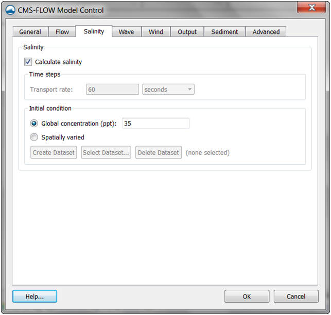
The salinity transport is activated within the CMS-Flow Model Control window (see figure below).
Figure 2-70. Salinity tab in the CMS-Flow Model Control window in SMS 11.1.
The CMS card used to turn on or off the salinity transport is described in Table 2-68.
Table 2-65. CMS card used to turn On or Off the salinity transport
| Input | Format | Notes |
|---|---|---|
| Salinity
Transport Activation |
[card=CALC_SALINITY_TRANSPORT]
[name=SalTrans, type=char, options=(ON,OFF), default=OFF] |
Turns on or off the salinity transport calculation. |
| Salinity
Transport Time Step |
[card=SALINITY_CALC_INTERVAL]
[name=SalTransdt, type=float, default=1.0, dependency=] [name=SalTransdtUnits, type=char, options=TimeUnits), default=’s’] |
Specifies the salinity transport time step (interval). Only used for explicit temporal scheme. |


