User Guide 016
4 Surface Roller Model Setup
The surface roller model is run after each CMS-Wave and before each CMS-Flow run. It runs on the wave grid but is a separate model and module within the CMS. The surface roller model parameters are set within the CMS-Flow cmcards for convenience and the cards are described in the table below. For more information on the surface roller model see section Surface Roller.
Table 4-1. CMS-Flow cards related to the surface roller.
| Input | Format | Notes |
|---|---|---|
| Surface Roller Model activation | [card=CALC_ROLLER]
[name=RollModel, type=char, options=(ON,OFF), default=OFF] |
Turns On or Off the surface roller model. |
| Surface Roller Model
Dissipation Coefficient |
[card=ROLLER_DISSIPATION_COEFFICIENT]
[name=RollDissipCoef, type=float, dependence=(RollModel==ON), default=0.1, typical=(0.05>RollDissipCoef<0.15)] |
Specifies the roller dissipation coefficient. Controls the energy dissipation in the roller model. Higher values produce stronger dissipation and reduce the net effect of the roller. |
| Surface Roller Model
Efficiency Coefficient |
[card=ROLLER_EFFICIENCY_COEFFICIENT]
[name=RollEffecCoef, type=float, dependence=(RollModel==ON), default=0.5, typical=(0.5>RollEffecCoef<1.0)] |
Specifies the roller efficiency coefficient. Controls the amount of wave breaking energy which is transferred to the roller. A value of 1.0 indicates that all of the wave breaking energy is transferred to the roller. |
| Surface Roller Scheme | [cards=ROLLER_SCHEME,
dependence=(RollModel==ON)] [name=RollSch, type=char, options=(UPWIND1,UPWIND2), default=UPWIND1] |
Specifies the surface roller transport scheme. UPWIND1is a first-order upwind scheme and UPWIND2 is a second-order upwind scheme. |
Example 4 1. Specifying the surface roller cards
CALC_ROLLER ON !ON | {OFF} ROLLER_DISSIPATION_COEFFICIENT 0.1 !default = 0.1, range = 0.05-0.15 ROLLER_EFFICIENCY_COEFFICIENT 0.5 !default = 0.5, range = 0.5-1.0 ROLLER_SCHEME UPWIND1 !{UPWIND1} | UPWIND2
5 Coupling of CMS-Flow and CMS-Wave
Steering refers to the coupling process between CMS-Flow and CMS-Wave. In CMS-Flow versions v3.75 and older (explicit CMS-Flow), the steering was done by the SMS interface. The new inline CMS contains both CMS-Flow and CMS-Wave and performs the coupling process internally. In either, the steering process is similar. First the wave model is run twice at time zero to the first steering interval. The wave information is then interpolated on to the flow grid and the flow model is run from time zero to the first steering interval. The flow information is then interpolated on the wave grid and the wave model is run for the second steering interval and the process is repeated until the simulation is complete.
Before running steering, it is a good idea to test the CMS-Flow and CMS-Wave separately to make sure there are no problems with their grids, or input parameters. Once the CMS-Flow and CMS-Wave models have been setup properly and loaded in SMS, the steering can be initiated.
CMS Versions 4.0 and newer the steering process is done internally by the CMS. This means that that both CMS-Flow and CMS-Wave are contained within a single code or executable. Even though CMS-Flow and CMS-Wave use different grids, the two models are in a single code which facilitates the model coupling and speeds up the computation by avoiding communication files, variable allocation and model initialization at every steering interval. The inline CMS can be launched from the SMS Steering Wizard or as a command line with arguments specifying the input files and steering options. The table below describes the CMS-Flow cards used for the steering process in the inline CMS.
Table 5-1. CMS-Flow cards related to steering
Card Arguments Default Range Description| CMS-WAVE_SIM_FILE
WAVE_SIM_FILE |
character | none | none | File name including path for the CMS-Wave sim file. |
| STEERING_INTERVAL | real | none | none | Sets the recurring hot start output time. |
| WAVE_WATER_LEVEL | character | TIDAL_PLUS_VARIATION | LAST
TIDAL TIDAL_PLUS_VARIATION |
Determines the method used to calculate the water levels passed to the wave model. |
| FLOW_EXTRAPOLATION_DISTANCE | real | Calculated based on grid geometry | none | Determines the extrapolation distance used for flow variables on the wave grid. |
| WAVE_EXTRAPOLATION_DISTANCE | real | Calculated based on grid geometry | none | Determines the extrapolation distance used for wave variables on the flow grid. |
Notes:
- 1. For both the SMS steering and inline steering, the CMS-Wave input spectra need to be spaced at regular time intervals and begin at the same time as the CMS-Flow model.
- 2. The way variables are interpolated and extrapolated both in space and time are slightly different between the SMS steering and inline steering versions of CMS.
- 3. Currently, the inline version of CMS only contains the implicit CMS-Flow solution scheme. Therefore, if the user decides to switch from explicit to implicit solvers, the user must also use different executables.
- 4. The wave grid for most inlet and coastal cases will be not much longer alongshore than the flow model. If the wave model does not extend far enough, there are model parameters to smoothly interpolate the wave data to some distance alongshore in the flow model.
- 5. Because the grid boundary is often the location of a wave buoy, the cross-shore domain tends to extend further.
- 6. In some cases the best IJ location for the half-plane model may not be apparent, especially for open coasts. Often the degree of energy in the open ocean is dominantly from one direction or the other, and the i-direction should be aligned to that direction.
- 7. The maximum length of the steering interval is a function of the tide (i.e. range and type of cycle such as diurnal, semidiurnal, or mixed), wave conditions, and nearshore bathymetry. In general, larger tide ranges and semidiurnal tides require shorter steering intervals. Larger wave heights and storm events require smaller steering intervals. Nearshore bathymetry is gentle slopes also requires shorter steering intervals because it small variation in water depth can lead to a large change in the location of the breaker.
Interpolation Files
When running the inline CMS with flow and waves, the CMS steering module write out two files named:
- • Intpcoef_flwav.bin
- • Intpcoef_wavfl.bin
These files contain the interpolation information between the CMS-Flow and CMS-Wave grids. Because calculating the interpolation information can take several minutes, saving this information in files allows the model to quickly read this information and avoid their computation for subsequent runs when using the same CMS-Flow and CMS-Wave grids. When the model is restarted it will automatically detect these files and read them if the grids are the same size. If changes have been made to the grids but the grid size is the same, the steering module will not be able to detect the changes and the interpolation information will be incorrect. Therefore, it is recommended to delete the interpolation files every time a change is made the either the CMS-Flow or CMS-wave grid. In the future, this problem will be avoided by writing a counter to the CMS-Flow and CMS-Wave files every time a change is made to them from the interface.
6 Running CMS
Recommended Folder Structure
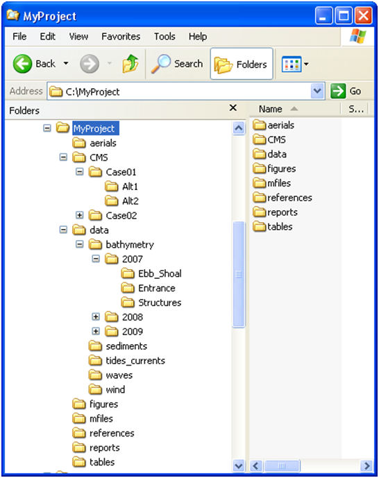
Any folder structure may be used. However, for purposes of organization and ease of use, it is recommended that a folder structure similar to that proposed here be used. For large modeling projects with many alternatives and simulations, a more complex folder structure may be warranted, but should be based on that below.
While the CMS accepts file names and paths with spaces, other software may have issues with spaces. Therefore, it is recommended that spaces are not used in the simulation path and filename without prior testing.
Figure 6-1. Recommended folder structure for CMS projects.
SMS CMS-Flow Menu
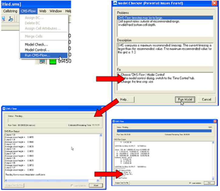
The first option for launching CMS versions 4.0 and newer is by simply running from the SMS CMS-Flow menu. If necessary the steering infor-mation can be entered in the advanced cards and CMS-Flow will automatically call CMS-Wave and perform the model coupling internally. The steps for running CMS-Flow from the SMS CMS-Flow Menu are outlined below.
- • Make sure both the CMS-Flow and CMS-Wave grids are loaded in SMS.
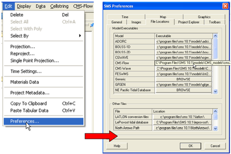
- • Check the CMS executable file name under the SMS preferences menu.
- 1. Click on Edit | Preferences.
- 2. Under the File Locations tab, in the section called Model Executables check the file names for CMS-Flow and CMS-Wave and make sure they are consistent with the latest re-leases (http://cirp.usace.army.mil/products/index.html CIRP Products).
Figure 6 2. Changing the CMS-Flow model executable.
- • Start CMS from the CMS-FLOW Menu
- 1. Click on CMS-FLOW | Run
- 2. In the SMS Steering Wizard select the CMS INLINE option and click on the Next> button.
- 3. Enter the Steering Interval under the Time section and click on the Start button.
Figure 6-3. Example of launching the CMS from the CMS-Flow menu.
Standalone Program
Standalone refers to the fact that the CMS executable is not part of a larger software package nor does it require a network connection, and support or services of the operating system or other software. If the CMS were run from the SMS it would not be considered a standalone program.
Because the inline CMS does all of the steering internally, it is a standalone program and there is really no need for CMS to be launched from SMS. Running CMS outside of SMS is useful because it allows the user to launch CMS from script files and also to pause the model for checking model results during the model simulation without causing access errors. When running several models, pausing the some of them will free up some of the computer to do other tasks such as plotting and checking model results. Running CMS outside of the SMS, also avoids the extra memory and work requirements from the interface.
There are three mean approaches for running CMS as a standalone program
- 1. From a command prompt
- 2. Double-click on the CMS executable or shortcut to the executable.
- 3. Drag-and-drop the CMS input files on the CMS executable or shortcut to the executable.
Notes:
- 1. For advanced users, it is recommended to put a copy of the CMS executable in the project directory and running the CMS from a command prompt. This keeps a record of the executable used for the project, facilitates making and transferring script files for running multiple project alternatives and keeps the window open after the model has completed or even crashed.
- 2. To pause the simulation, press the Pause/Break button on your keyboard or press and hold the “Ctl” key and press the “S” key.
- 3. To stop the model simulation, press and hold the Ctrl key and press the C key.
Opening a Command Prompt
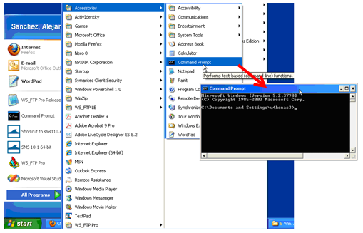
The first step is to open a command prompt. There are two ways of doing this:
The first method for opening a command prompt is
- 1. Click on Windows Start | Accessories | Command Prompt
Figure 6-4. Example of launching the inline CMS-Flow steering run.
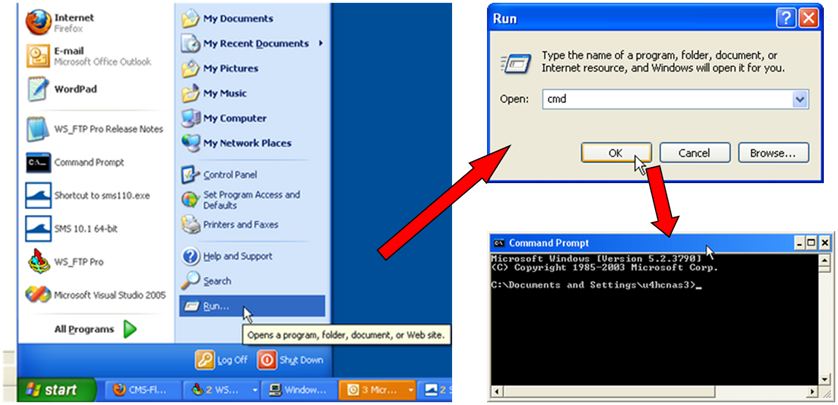
The second method for opening a command prompt
- 2. Click on Windows Start menu then the Run… utility
- 3. In the Run window, enter the command cmd and click OK
Figure 6-5. Example of launching the inline CMS-Flow steering run.
Note:
- • It is recommended to put a shortcut to the Command Prompt on the desktop to more easily open the Command Prompt.
Once the command prompt is open the CMS can be launched using one of the following syntax
- >> [cms2d_*exe] [*.sim or *.cmcards file] [*.sim or *.cmcards file] [steering interval] [wave water level option]
where the steering interval is in hours and the wave water level option is either
- 1. Wave water levels are estimate as the last water levels from the flow model (i.e. WAVE_WATER_LEVEL option equal to LAST)
- 2. Wave water levels are estimated as the mean tidal water level at the wave time step (i.e. WAVE_WATER_LEVEL option EQUAL TO TIDAL).
- 3. Wave water levels are estimated as the mean tidal water level at the wave time step plus the water surface variations estimated from the last flow time step (i.e. WAVE_WATER_LEVEL option EQUAL TO TIDAL_PLUS_VARIATION).
Notes:
- • The *.sim and *.cmcards files must contain the full or relative path with respect to the executable if different from the executable.
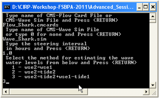
- • If no input arguments are specified, than the user will be prompted to manually enter the name of the CMS-Flow and CMS-Wave files and steering information.
- • If the cmcards file is specified the CMS will check for the steering cards. If the sim file is found, than it will run in steering.
- • If no steering interval is specified in the cmcards file or the com-mand line, than a default value of 3.0 hours will be used.
- • If no wave water level option is specified in the cmcards file or the command line, than a default method equal to three.
- • It is possible to create a short-cut to the model executable and simply drag-and-drop the cmcards file and or sim file with the steering options specified in the cmcards file.
Below are some examples
- >> cms2d_v4p1r19-x64p.exe
- >> cms2d_v4p1r19-x64p.exe Flow.cmcards
- >> cms2d_v4p1r19-x64p.exe Flow.cmcards Wave.sim
- >> cms2d_v4p1r19-x64p.exe Wave.sim Flow.cmcards
- >> cms2d_v4p1r19-x64p.exe Flow.cmcards Wave.sim 1.0
- >> cms2d_v4p1r19-x64p.exe Wave.sim Flow.cmcards 3.0 1
Drag-and-Drop
To launch CMS as a standalone application using the drag-and-drop method:
- 1. Select all of the CMS input files by holding the Ctrl key and single-clicking on each input file.
- 2. Drag all of the input files on the CMS executable or shortcut to the executable by holding the left mouse button.
- 3. Drop the files by letting go of the left mouse button.
Note:
- • If running steering, make sure all of the steering options are in the cmcards file when using the method.
Double Click
This is one of the easiest ways of running the CMS but also one of the most time consuming because it requires the user to type the name and path (if different from executable) for all of the input files and if necessary the steering options.
- • To run the CMS by using the Double-Click method:
- 1. Double-click on the executable
- 2. Follow the instructions on the screen.
Figure 6-6. Example of launching the inline CMS by double-clicking on the executable.
Note:
- • If CMS input files are not in the same folder as the executable, the file
Windows Priority Levels
In Windows NT/2000/XP/7 it is possible to assign a process a different priority level using the Task Manager. This is useful for running CMS in the “background” without slowing down the computer. Windows NT offers three different priority levels while Windows 2000/XP/7 offers five. The priority level can be set when launching the executable from a Command Prompt or batch file or changed after the model is started from the Task Manager. To set the priority level from the Command Prompt use one of the following switches /low, /belownormal, and /abovenormal.
When initiating CMS simulations from a batch file, precede each of the lines in the above example with “start "CMS" /wait /low” as shown below. This initiates a separate Console Window for each simulation on a low priority. You can also see which simulation is active by viewing the primary Console Window. The /wait option is necessary to force the next simulation not to start until the current one is complete. It is not recommended to use /high priority since this may cause the machine to freeze up. To change the priority level of simulation manually, open Task Manager (see your System Administrator if you’re not sure how to do this), click on the Processes Tab and find the CMS executable process you wish to change, right click on the process, choose Set Priority, then set the priority.
7 Viewing and Post-Processing Results
Calibration of hydrodynamic and morphologic datasets requires use of post-processed data in order to compare to measurements and make incremental changes. This section gives guidance on how to process or extract data from model results, and examples of measured data to compare results with. Of course, the post-processed data can be exported and comparisons can be made in another program, but there are some options within SMS that can help with repetitive testing and comparisons.
Water Levels & Currents
The first stage in calibration of a numerical hydrodynamic model is to accurately represent measured tides (or water levels) and currents. The number of calibration measurement sites required for sufficient model calibration increases with larger domains and increased complexity in processes.
Of the three main data sources required for good hydrodynamic calibra-tion (geomorphic, forcing, and field data), inaccurate knowledge of, or mistakes in conversion between datums is the most common underlying factor in poor model calibration. Model calibration cannot be achieved without proper representation of datums. Some examples of field data typically used for calibration of hydrodynamics include fixed water level gauges, fixed acoustic Doppler velocimeters (ADV) and acoustic Doppler current profilers (ADCP), and roaming or boat-mounted ADCPs. Both fixed and roaming data can be assessed over a time series, where boat-mounted data are collected at specified locations over time intervals. However, roaming data that were collected continuously must be assessed as a function of location in three-dimensional space.
For hydrodynamic data, the most common forms of measurements are recorded either temporally at a station, temporally at a fixed spatial extent, or spatially at relatively singular times. For example, a tide gage is stationary, but a horizontal acoustic Doppler current meter (H-ADCP) may collect temporal measurements at multiple points. Of course, the multiple locations are depth-averaged, as would be an upward-looking ADCP, in order to compare to the 2D CMS. Similarly, a field campaign of depth-averaged current measurements collected at transects are all contemporaneous (within reason), but there are multiple time periods to compare.
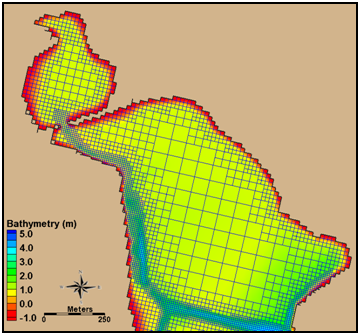
With good forcing data and accurate corresponding datums, the final check before hydrodynamic calibration can be achieved is the accuracy and detail of the geomorphic parameters such as bathymetry, sediment characterization, and structure definition. The most important of these is bathymetry, which can have several issues which are typically associated with quality control, density, interpolation, and final grid resolution and domain size. A good example of this is a poorly resolved small channel in the far reaches of a bay, such as that in the northern portion of the Shark River estuary (Figure 4-51). Although lower velocities may be passing through this channel, and there may be little interest in morphology change here, it may be integral to providing the conduit of tidal prism to a shallow bay platform.
Figure 7-1. Northern portion of the Shark River estuary
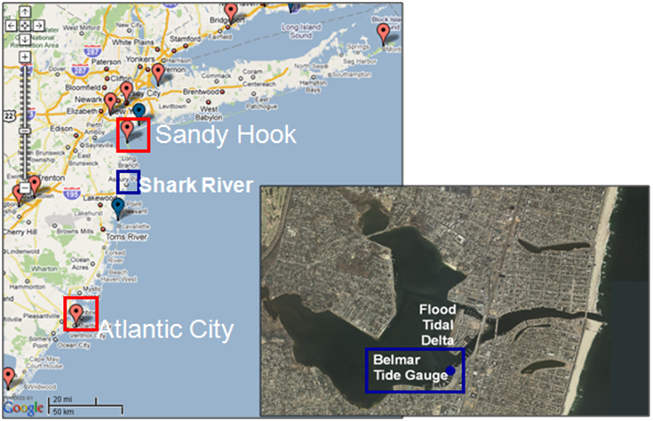
Figure 4-53 shows the closest locations of water-level gauges to Shark River Inlet. Sandy Hook and Atlantic City, NJ, are two ocean pier-mounted gauges approximately 30 and 100 miles away from Shark River Inlet, respectively. Both NOAA gauges were evaluated against the Belmar tide gauge using the tidal constituents of one year, and Sandy Hook was found to have the closest amplitudes and phases. Measured tides from Sandy Hook were used to force the offshore boundary condition. The calibration period that the model was evaluated on was for the 13-hour tidal cycle over which field measurements were collected on 20 August 2009.
Figure 7-2. Location of NOAA (red) and USGS (blue) water level gauges.
Display Options
The results of the CMS calculated hydrodynamics can be viewed and compared to measured results in a number of ways. Scalar results are typically in planar view and are illustrated by color representing magnitude, and arrow lengths representing magnitude and direction. Color setting can be manipulated in the overall Display Options, or individually for each dataset.
- 1. Open a solution file for the hydrodynamic output and right click on the WSE dataset, select Display Options.
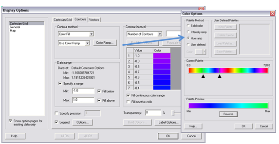
- 2. In the Contours tab, adjust the color settings and the value range to that in Figure 4-53.
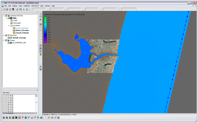
Figure 4-54 illustrates the new color scheme for displaying the water surface elevation.
Figure 7-3. Contour tab settings for color display and value range. Note the blue colors were selected for the visible range.
Figure 7-4. Water surface elevation color contours modified
Currents are automatically given in vector format as the solution files are generated. These can be converted into Vx and Vy components, or into magnitude and direction. If the modeled results are compared to simple magnitude measurements, then the magnitude dataset is appropriate. If the modeled results will be compared to measurements collected in east-ing and westing, care should be taken to compare the correct derivative of the vector format. Because the vectors are based on the Cartesian grid’s orientation, be sure to convert with respect to the axis difference.
- 1. Right click on the current vector dataset and select Vector to Scalar. Select Vx and Vy, and this gives the x and y compo-nents of the current velocity.
- 2. Next, convert the vector to Magnitude and Direction. The color component of the magnitude can be selected along with the vector of the current velocity.
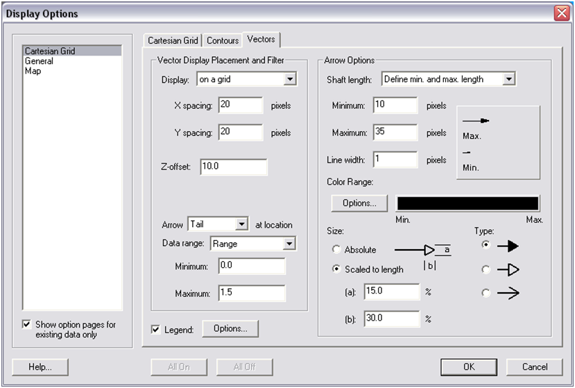
- 3. Open the Display Options, and go to the Vector tab. Change the vectors to the below settings (Figure 4-55) to view the vectors over a prescribed gridding. (Note that individual vectors at each cell is difficult to visualize for the whole domain and often only useful when zoomed in very close.)
Figure 7-5. Vector Display options set for a gridded display across the domain.
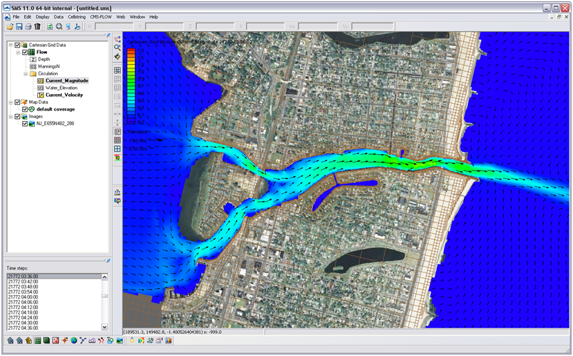
Figure 4-56 shows an example of displaying current magnitudes with color contours and the current direction with vectors.
Figure 7-6. Vectors and color contours set for displaying current magnitude (color) and direction (vectors). Note that the vectors are slightly scaled on this setting to reflect magnitude.
Importing water level measurements into SMS for comparison
To compare the measured data within SMS, the measurements must be brought into the program and into a comparable format. SMS will import a variety of ASCII, columnar data that can be categorized and labeled in a scatter dataset (scatterset).As a simple example of comparing tidal data to calculated tides, the USGS Belmar tide data is given in the folder Hydro\Water Level Calibration in the Tide_Comparison_AUG09_Workshop.xls file. This is the only tide measurement for Shark River Estuary to compare the bay tidal harmonics. To import this data, it must be brought in as observational data within the Observation Map Module.
- 1. In the Cartesian Module, go to Display, Plot Wizard, and select Time Series Plot. Select scalar, and the WSE as the dataset. (Note it takes some time to populate a plot in SMS.)
- 2. Change the map module Default Coverage type to Observation, and add a Feature Point
 to the approximate location of the tide gauge shown in Figure 4-57.
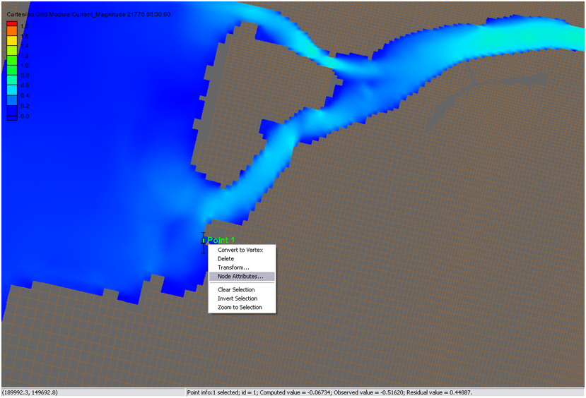
 - 3. Right click on this feature point (Figure 4-57), and select attributes.
Figure 7-7. Observation point placed at the location of the Belmar tide station.
4. In the Attributes, check the Trans box in measurements, and select 2D Cartesian under Module, and the Water_Elevation dataset (Figure 5-58). If your Observe Point is checked, an Options box should appear under the Time Series column. Select this and import the Belmar_Tide.xys file.
Time series of the measured water levels can be manually pasted here. A file of measured water levels is provided and available for Import: Belmar Tide Input.tsd.
