User Guide 018
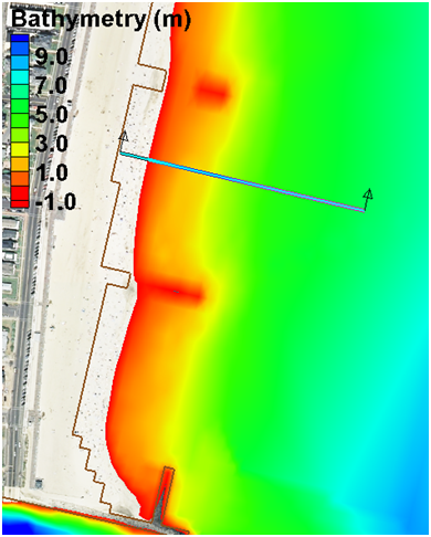
Figure 7-30. Highlighted Feature Arc with the positive direction shown by the arrows.
- 5. If necessary, the arc direction may be changed by clicking on the Select Feature Arc
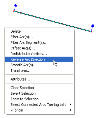
 tool, and selecting the feature arc by right-clicking it once and selecting the option: Reverse Arc Direction (see figure below). The same applies for feature polygons.
Figure 7-31. Reversing the arc direction.
The net sediment transport dataset is integrated along the arc (line inte-gral) to compute the sediment transport across the Feature Arc. This pro-cedure is done in the SMS Plot Wizard. The sediment transport vector field is interpolated to the points where the arc intercepts cell faces and is then integrated across the Feature Arc. Follow each step outlined below:
- 6. Open the Plot Wizard by clicking on the plot wizard icon
 , or clicking on the Display menu and selecting Plot Wizard.
 - 7. Select Time series as the Plot Type and then click Next.
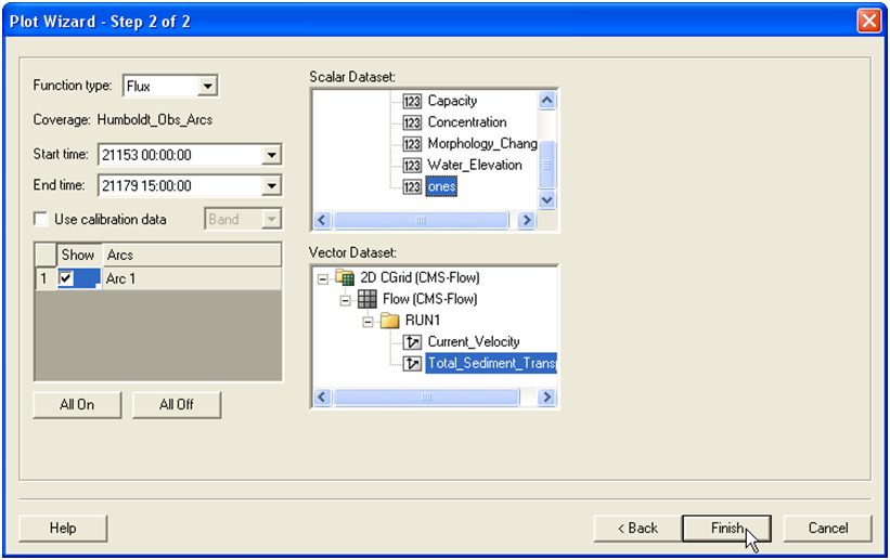
- 8. In the Plot Wizard – Step 2 of 2 window, select Flux as the Function type.
- 9. Check the appropriate feature arc checkbox(es).
- 10. Select the ones dataset for the scalar dataset.
- 11. Select the Sed_Tranp_Net as the vector dataset.
- 12. Make sure the start and end times are correct.
- 13. Select Finish.
Figure 7-32. Selecting the correct Start and End Times, Feature Arcs, and Scalar and Vector Datasets in Step 2 of 2 of the Plot Wizard.
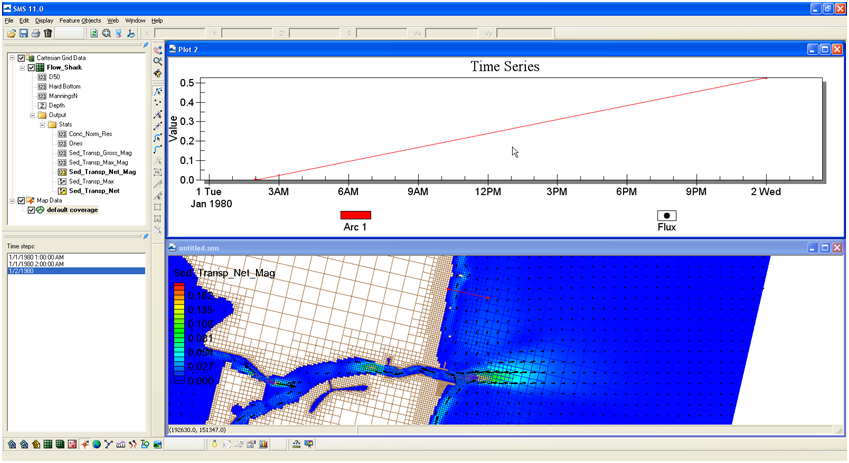
A plot will appear in SMS similar to the example shown below
Figure 7-33. Example plot of an integrated net sediment transport rate across a feature arc.
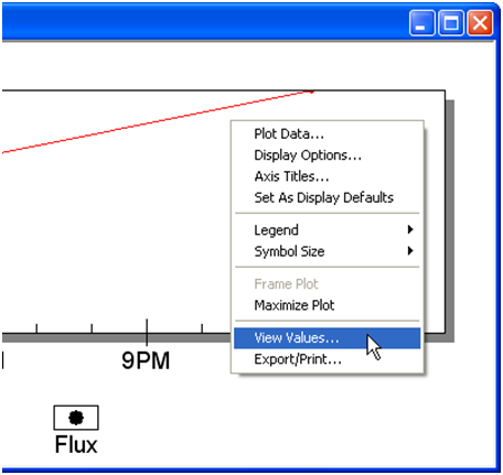
To view the final value of the net sediment transport rate across the fea-ture arc, left-click on the plot, and select View Values… (see figure below).
Figure 7-34. Selecting View Values… after left-clicking on the time series plot.
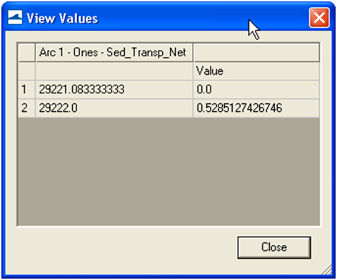
An SMS window will appear with the title View Values. The net sediment transport rate across the feature will be shown under the second row un-der the Value column. The units of the transport will be kg/s.
Figure 7-35. Net sediment transport rate integrated across
Morphology
The results of the CMS calculated morphology change can be visualized several ways, from three dimensional or planar view of the bathymetry, planar view of the volumetric erosion and accretion, and with 1-D cross-sections of the time series. All vector and scalar information can be ex-tracted from points and arcs (and polygons) in SMS. This section will cover the methodology used to post process time series morphology change data.
To plot channel infilling in SMS in a graphical format, the results in the solution file need to be changed from depths (the depth below the datum in which CMS calculates) to elevations. SMS can plot multiple cross-sections, or arcs, against each other, or through time.
Channel Infilling by cross-sections
- 1. Load Jan09tel.cmcards (and solution file, if it does not load auto-matically).
- 2. Right-click on the Time Series window on the left and select “Time Settings”, and change the time reference from Relative to Absolute.
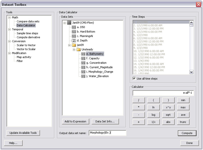
- 3. In the Cartesian Grid Module, click Data, Data Calculator, and the Data Calculator should be selected in the Tools section as shown in Figure 7-36.
- 4. Select the Bathymetry scalar (
 ) dataset; under Time Steps check the Use all time steps on, and double-click the Bathymetry.
 - 5. The line under Calculator will display “e:all”, add the multiplication symbol (*) and negative 1 (-1) as shown in Figure 7-18.
- 6. Change the Output data set name as shown in Figure 7-18 so as to distinguish this dataset from the original Bathymetry output, click Compute, and after the scalar set appears in the SMS window, click Done. (Note: values for the contours may need to be adjusted to view elevation range.)
Figure 7-36. Data Calculator Options in the Dataset Toolbox.
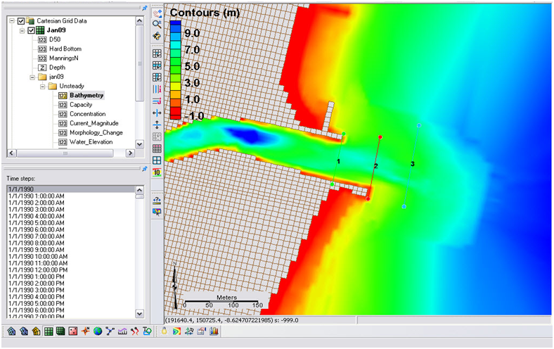
Figure 7-37. Display of calculated bathymetry now converted to elevations. Note the legend has been modified to display the new contours.
- 7. Create feature arcs for extracting the time series data by switching to the Map Module button
 , or Map Data
  , rt-click on default coverage, and select Type, Generic, Observation
 - 8. Click the Create a Feature Arc button
 to generate the arcs from which cross sections will be extracted, and click on one side of the channel and double-click on the other side to close the arc
 - 9. Click the Select a Feature Arc
 button and select the generated arc (Note that there is a direction associated with the arc, which determines the sideview of the cross section)
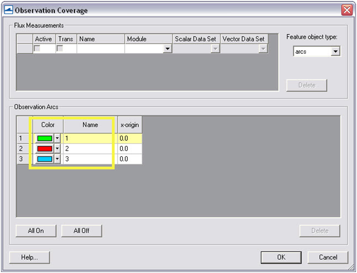
 - 10. Right-click an arc and click on Attributes, and set the color and name(s) of each arc which are listed together in the Observation Coverage options (Figure 7-38), click OK.
Figure 7-38. Observation Coverage attributes
- 11. To plot the profiles in SMS, Select Display, Plot Wizard, and Observation Profile, and select Next.
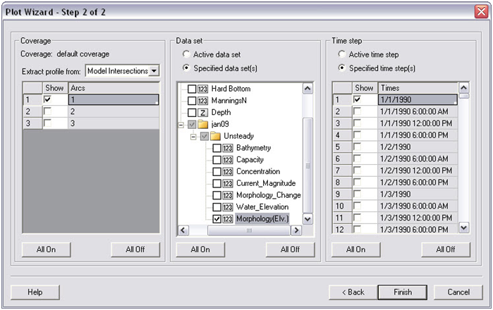
- 12. Following Figure 7-39, under Coverage check one arc (though multiple can be plotted), under Data set select Specified data set(s) and select the generated Morphology (Elev.) set only, and under Time step select Specified time step(s) and check on several times spaced apart by at least several days to months, click Finish.
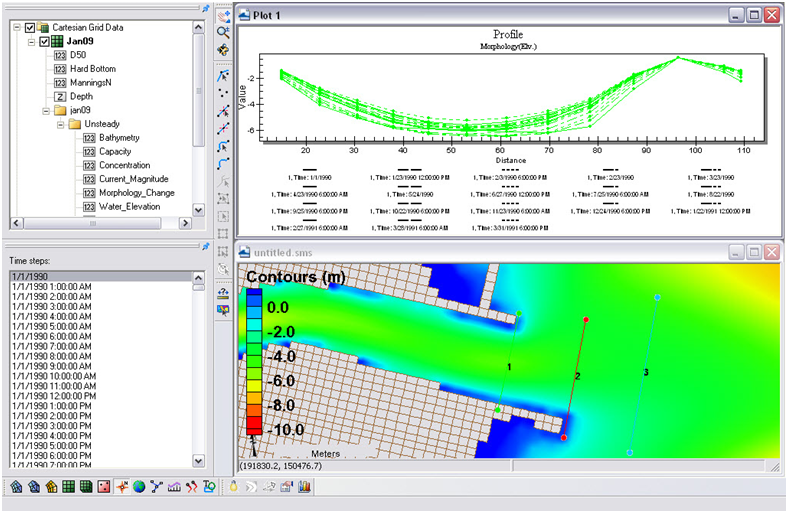
- 13. Right-click on the plot (Figure 7-40) and select view values.., and a table will appear with all the plotted distance and elevations given in the graph, (Note this ASCII table can be copied and pasted into EXCEL).
Figure 7-39. Plot Wizard Step 2.
Figure 7-40. Plotted cross-section.
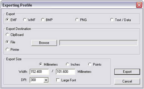
- 14. To export the data in different formats, right-click on the plot, and select Export/Print for several options to export the graph or data from the graph (Figure 7-41)
- 15. To add more profiles or time-series, right-click on the plot, and select Plot data.. to bring up the original options from Figure 7-40.
Figure 7-41. Data Export Options.
Analysis of cross-sectional area and sediment volume changes are the most common approaches to quantifying morphologic change. Another method of quantifying change in a spatial framework is through compari-son of the planform aerial change. This method is useful in delineating active zones of transport, typically based off of the depth of closure, and can define the upper and lower limits of transport. These results can be used to interpret bypassing areas or zones, however, determining the by-passing pathways should not be based off of this analysis alone.
Planform area changes
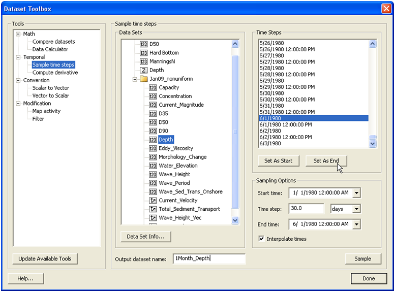
- 1. To filter the morphology dataset for the time periods of interest, i.e. every month, open the Data Calculator and select Sample time steps under the Temporal section (Figure 7-42).
Figure 7-42. Sampling time steps from a solution dataset.
- 2. Select Depth under Data Sets, change the Output dataset name, and set the start time and end time to Jan 1 and Jun 1, respectively, with an interval of 30 days. Select Sample. This should produce a Depth time step approximately every month.
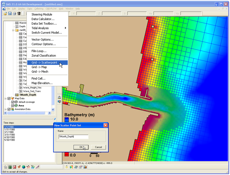
- 3. In order to map an elevation, the grid must be converted to a scatterset.
- • Rather than take the time required to convert the en-tire solution during this workshop, we have provided this file in the folder (File: 1Month_Depth). (To con-vert the grid solution file to a scatterset, select Data|Map to Scatter, and SMS will convert all of your time series datasets to the scatter module (Figure 7 43). This can take anywhere from minutes to hours, depending on the size of the file and speed of the processor. Open the provided scatterset.
- • Or, delete the Jan09_nonuniform solution datatree so that the main CMS-Flow datasets and the 1Month_Depth dataset are the only datasets left. Then select Data|Grid-> Scatter, and SMS will convert only those datasets.
Figure 7-43. Converting a solution dataset to a scatter dataset.
- 4. Create a new map coverage (by right clicking Map Data in the data tree and selecting New Coverage) for mapping out specified contours over the time series depth scatterset.
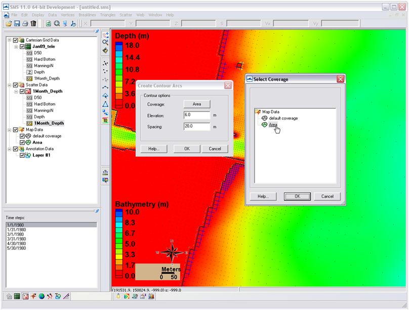
- 5. Select the 1Month_Depth Scatterset (Scatter Module should be on) and the first time stamp (1 Jan), and go to Data|Scatter Contour -> Feature. Choose an elevation to map (6.0 m), a spacing of the points in the resultant arc, and select the Map Coverage (‘Area’ in Figure 7-44) that the arcs are created in.
Figure 7-44. Mapping a scatterset contour to the map module.
- 6. Create another new Map Coverage, select the final timestamp (30 May), and go to Data|Scatter Contour -> Feature and select the same elevation (6.0 m) and point spacing. Switch between the two coverages to view the location of each contour (Figure 7-45). Note that the arcs hold a z-elevation (displayed in Z in the bar above) and are partially visible under the color-filled scatter data.
Figure 7-45. Mapped coverage of the 6-m contour at Months 1 and 6 (left and right, respectively).
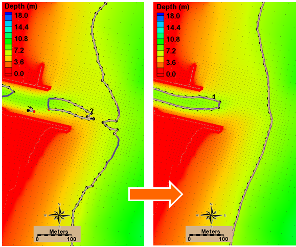
- 7. To calculate planform area, each contour in both maps must be closed off with arcs to create a polygon. Create a polygon in the closed arcs by selecting Feature Objects|Build Polygons. An example is shown in Figure 7-46. Note that the area of the selected polygon is given at the bottom of the screen in the units the solution file is given in, which is always metric for the CMS.
Figure 7-46. Left: Two arcs drawn to connect the 6m contour back to a common point to close off the polygon. Right: Highlighted polygon after created.
Creating polygons between time series allows for calculation of planform area change at a morphologic spatial scale through time. The difference shown in the arcs is substantial, and can be quantified with the use of arcs and polygons. It is important to be careful with delineating the morphologic form of interest. If the full area is being calculated for a feature (an ebb shoal), be sure to be discrete in the size of these aerial calculations because they may skew the final calculation of the morphologic feature of interest.
Similarly, volume change can be elicited from polygons created with Feature Arcs. The next section describes how to calculate volume change over an arc.
Calculating volume change from polygons.
- 1. Create a polygon similarly to the above exercise that created arcs to complete a polygon in the planform area calculations. Choose an area around the ebb shoal, or within the channel, and draw a single arc connecting around the feature. Be sure to close the end of the polygon by letting the mouse automatically hover over the final point (the pointer will relocate when placed near another feature point).
- 2. Create a polygon in the closed arcs by selecting Feature Objects|Build Polygons. An example is shown in Figure 7-46.
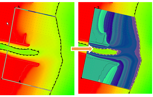
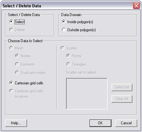
- 3. To select the cells within the polygon, next, with the polygon selected, go to Feature Objects|Select/Delete Data, and select select, Cartisian Grid Cells, and Inside Polygon (Figure 7-47).
Figure 7-47. Options for selecting and deleting data from Mesh, Cartesian Grids, and Scattersets using polygons.
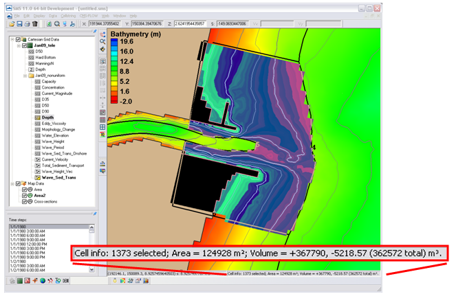
Note, again, that the volume of the selected polygon is given at the bottom of the screen in the units the solution file is given in, which is always metric (m3) for the CMS. The volume given in the lower right corner of the window (Figure 7-48) are a positive, negative, and total volume representative of the integrated positive, negative, and combined volumes from each cell. Therefore, the numbers represent the volume based off of the dataset’s datum.
Figure 7-48. Selected cells from a polygon. Volume information given in lower, right corner of screen.
If depths are selected in the solution datatree as the measurement for volume calculation (one of the direct outputs in the CMS solution file), volume is positive and represents the space that the water occupies. To get the volume of a morphologic feature, a base level to calculate above must be chosen. Navigation depths or depth of closures are often used as a base level for a quick estimation of volume. The area of the cells is also included in basic cell info at the bottom of the screen, as illustrated in Figure 7-48. Multiplying this area by the base level (with respect to the model datum) will produce a base volume of which the calculated volumes can be subtracted from.
