User Guide 024

13 Appendix C: Matlab Scripting

Scipting refers to the automation of running multiple CMS runs with dif-ferent parameters, without manually having to create and edit each alternative. The scripting process can include the following steps:

1. Setting up alternatives

2. Creating batch file

3. Plotting and analyzing results

Scripting can be done using a variety of software programs. The examples shown here were written in Matlab because it is widely used, easy to read and convenient for plotting and analyzing results.

Setting Up Alternatives

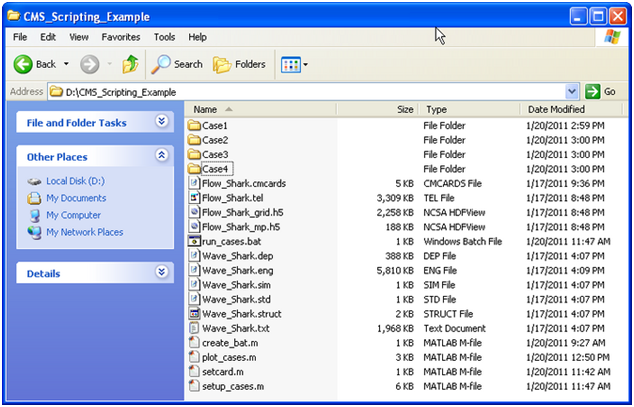
‎In this example, 4 cases or alternatives (Figure 5.11.1) are set up using the Matlab script below. The script copies the base setup files into subfolders and then modifies specific CMS-Flow cards in the *.cmcards file. The set-tings for each case are setup using a structure variable with field names corresponding to each CMS-Flow card (e.g. TIME_SERIES_INCREMENT). Separating each case into its own subfolder keeps the input and output separate and also allows for the different cases to be run at the same time.

Figure D-1. Example of scripting showing the files used.

---

% Matlab Script: setup_cases.m clear all flow = 'Flow_Shark'; wave = 'Wave_Shark'; ncases = 4; %Number of cases or alternatives r(1).MANNINGS_N_DATASET = '"Manning_Alt1.h5" "Flow_Shark/Datasets/ManningsN"'; r(1).WAVE_CURRENT_MEAN_STRESS = 'W09'; r(1).TIME_SERIES_INCREMENT = 1800; r(2).MANNINGS_N_DATASET = '"Manning_Alt1.h5" "Flow_Shark/Datasets/ManningsN"'; r(2).WAVE_CURRENT_MEAN_STRESS = 'DATA2'; r(2).TIME_SERIES_INCREMENT = 900; r(3).MANNINGS_N_DATASET = '"Manning_Alt2.h5" "Flow_Shark/Datasets/ManningsN"'; r(3).WAVE_CURRENT_MEAN_STRESS = 'W09'; r(3).TIME_SERIES_INCREMENT = 900; r(4).MANNINGS_N_DATASET = '"Manning_Alt2.h5" "Flow_Shark/Datasets/ManningsN"'; r(4).WAVE_CURRENT_MEAN_STRESS = 'DATA2'; r(4).TIME_SERIES_INCREMENT = 600; for i=1:ncases

 d = ['Case',int2str(i)];
 if ~exist(d,'dir')
   mkdir(d)
 end
 copyfile([wave,'.*'],d)
 copyfile([flow,'.*'],d)
 copyfile([flow,'_mp.h5'],d);
 copyfile([flow,'_grid.h5'],d)
 cards = fieldnames(r(i));
 file = ['.\',d,'\Flow_Shark.cmcards'];
 fork=1:length(cards)
   setcard(file,cards{k},r(i).(cards{k}));
 end

end return

---

The script above requires the subroutine below.

---

function setcard(cmcardsfile,card,value) % setcard(file,card,value) % Overwrites or appends a CMS-Flow card % in the *.cmcards file copyfile(cmcardsfile,'temp') fid=fopen('temp','r'); fid2=fopen(cmcardsfile,'w'); nc=length(card); ok = false(1); if ~ischar(value)

 value = num2str(value);

end while 1

 tline = fgets(fid); 
 if ~ischar(tline), break, end
 if strncmp(card,tline,nc) 
   fprintf(fid2,'%s       %s %s' ,card,value,tline(end));
   ok = true(1); 
   continue 
 end 
 nline = length(tline); 
 if(~ok && strcmp(tline(1:min(nline,14)),'END_PARAMETERS')) 
   fprintf(fid2,'%s       %s %s',card,value,tline(end)); 
   fprintf(fid2,'%s' ,tline);        
   break 
 end
 fprintf(fid2,'%s' ,tline);

end fclose(fid); fclose(fid2); delete('temp') return

---

Creating a Batch File

Although it is possible to launch CMS from Matlab a batch file is prefera-ble to use a batch file because it allows running all of the cases without opening Matlab.

---

% Matlab Script: create_bat.m cmsexe = 'cms2d_v4r23_x64p.exe'; %CMS-Flow executable batfile = 'run_cases.bat'; %Output batch file numgroup = 2; %Number of cases to run in a group fid = fopen(batfile,'w'); for i=1:ncases

 cmcards = ['.\Case',int2str(i),'\',flow,'.cmcards']; %cmcards file
 if mod(i,numgroup)~=0
   fprintf(fid,'START       %s %s %s',cmsexe,cmcards,char(10)); 
 else
  fprintf(fid,'START /WAIT %s %s %s',cmsexe,cmcards,char(10));
 end

end fclose(fid); return

---

The following text shows what the resulting batch file (*.bat) looks like

---

START cms2d_v4b42_x64p.exe .\Case1\Flow_Shark.cmcards

START /WAIT cms2d_v4b42_x64p.exe .\Case2\Flow_Shark.cmcards

START cms2d_v4b42_x64p.exe .\Case3\Flow_Shark.cmcards

START /WAIT cms2d_v4b42_x64p.exe .\Case4\Flow_Shark.cmcards

---

To run the batch file, simply double click on the file and each case will launch separately in its own MS-DOS window.

Plotting

The following example reads the Observation Point time series output file (*_eta.txt) and plots the 3rd column corresponding to the second observation point.

---

% Matlab Script: plot_cases.m close all eta = cell(ncases,1); for i=1:ncases

 etafile = ['.\Case' ,int2str(i),'\',flow,'_eta.txt' ]; %Water elevation
 eta{i} = load(etafile);    

end figure hold on for i=1:ncases

 h = plot(eta{i}(:,1),eta{i}(:,3),'-');  %3 is the index is the observa-tion point index

end ylabel('Water elevation, m') xlabel('Elapsed Time, hr') return

---